- Data Professor
- Posts
- How to Build a Machine Learning App in Python
How to Build a Machine Learning App in Python
Step-by-step tutorial from scratch in < 150 lines of Python code
Chanin Nantasenamat
May 27, 2021

Have you ever wished for a web app that would allow you to build a machine learning model automatically by simply uploading a CSV file? In this article, you will learn how to build your very own machine learning web app in Python in a little over 100 lines of code.
The contents of this article is based on a YouTube video by the same name that I published a few months ago on my YouTube channel (Data Professor), which serves as a supplementary to this article.
Importance of model deployment
Before diving further let’s take a step back to look at the big picture. Data collection, data cleaning, exploratory data analysis, model construction, and model deployment are all part of the data science life cycle. The following is a summary infographic of the life cycle:

Data science lifecycle. (Drawn by Chanin Nantasenamat aka Data Professor)
It is critical for us as Data Scientists or Machine Learning Engineers to be able to deploy our data science projects in order to complete the data science life cycle. The deployment of machine learning models using established frameworks such as Django or Flask may be a daunting and/or time-consuming task.
Overview of the Machine Learning App
At a high-level, the web app that we will be building today will essentially take in a CSV file as input data and the app will use it for the construction of a regression model using the random forest algorithm.
Now, let take a granular look at the details of what is happening at the front-end and back-end of the web app.
Front-end
Users are able to upload their own dataset as CSV file and they are also able to adjust the learning parameters (in the left panel) and upon adjustment of these parameters, a new machine learning model will be built and its model performance will then be displayed (in the right panel).
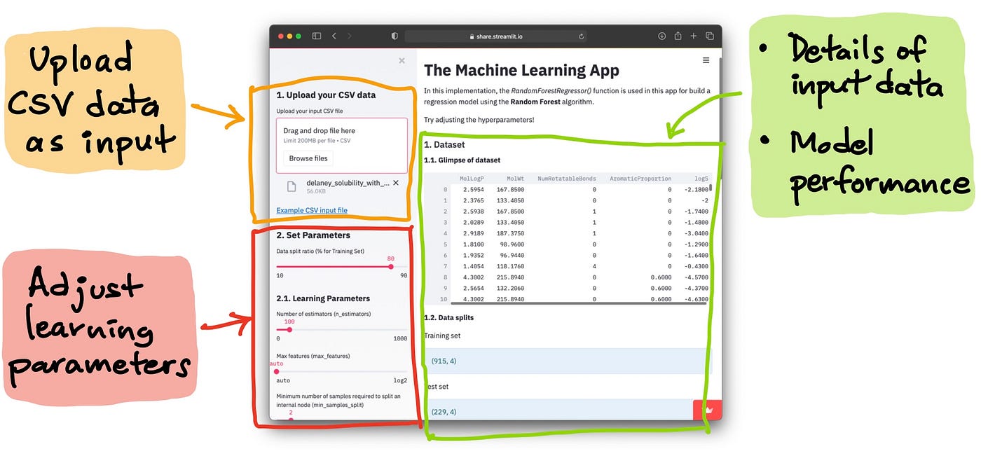
Anatomy of the machine learning app. The left panel accepts the input and the right panel displays the results.
Upload CSV data as input
The CSV file should have a header as the first line (containing the column names) followed by the dataset in subsequent lines (line 2 and beyond). We can see that below the upload box in the left panel there is a link to the example CSV file (Example CSV input file). Let’s have a look at this example CSV file shown below:
MolLogP,MolWt,NumRotatableBonds,AromaticProportion,logS
2.5954000000000006,167.85,0.0,0.0,-2.18
2.376500000000001,133.405,0.0,0.0,-2.0
2.5938,167.85,1.0,0.0,-1.74
2.0289,133.405,1.0,0.0,-1.48
2.9189,187.37500000000003,1.0,0.0,-3.04
Adjust learning parameters
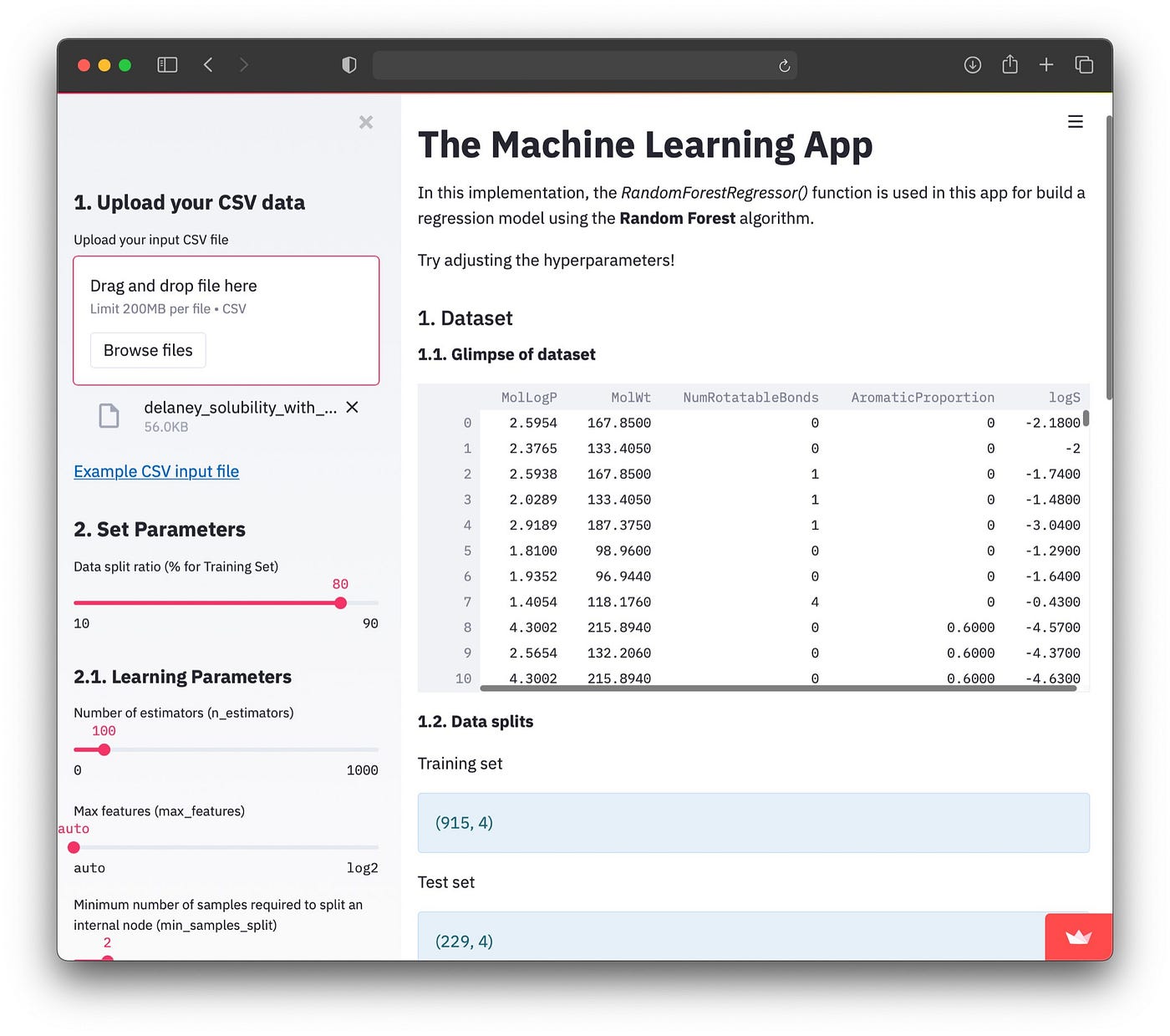
After uploading the CSV file, you should be able to see that a machine learning model has been built and its results are displayed in the right panel. It should be noted that the model is built using default parameters. The user can adjust learning parameters via the slider input and with each adjustment a new model will be built.
Model output (right panel)
In the right panel, we can see that the first data being shown is the input dataframe in the 1. Dataset section and their results will be displayed in the 2. Model Performance section. Finally, learning parameters used in the model building is provided in the 3. Model Parameters section.
Model built upon uploading the input CSV file.
As for the model performance, performance metrics are shown for the training set and test set. As this is a regression model, the coefficient of determination (R^2)and error (either the mean squared error or mean absolute error).
Back-end
Now, let’s take a high-level look under the hood of the inner workings of the app.
Upon uploading the input CSV file, the contents of the file will be converted into a Pandas dataframe and assigned to the df variable. The dataframe will then be separated into the X and y variables in order to prepare it as input for Scikit-learn. Next, these 2 variables are used for data splitting using the user specified value in the left panel (by default it is using the 80/20 split ratio). Details on the data split dimension and the column names are printed out in the right panel of the app’s front-end. A random forest model is then built using the major subset (80% subset) and the constructed model is applied to make predictions on the major (80%) and minor (20%) subsets. Model performance for this regression model is then reported into the right panel under the 2. Model Performance section.
Tech Stacks used in this Tutorial
This will be carried out using just 3 Python libraries including Streamlit, Pandas and Scikit-learn.
Streamlit is a simple to use web framework that allows you to quickly implement a data-driven app in no time.
Pandas is a data structure tool that makes it possible to handle, manipulate and transform tabular datasets.
Scikit-learn is a powerful tool that provides users the ability to build machine learning models (i.e. that can perform various learning tasks including classification, regression and clustering) as well as coming equipped with example datasets and feature engineering capabilities.
Line-by-Line Explanation
The full code of this app is shown below. The code spans 131 lines and white spaces are added along with commented lines in order to make the code readable.
import streamlit as st
import pandas as pd
from sklearn.model_selection import train_test_split
from sklearn.ensemble import RandomForestRegressor
from sklearn.metrics import mean_squared_error, r2_score
from sklearn.datasets import load_diabetes, load_boston

#---------------------------------#
# Page layout
## Page expands to full width
st.set_page_config(page_title='The Machine Learning App',
    layout='wide')

#---------------------------------#
# Model building
def build_model(df):
    X = df.iloc[:,:-1] # Using all column except for the last column as X
    Y = df.iloc[:,-1] # Selecting the last column as Y

    # Data splitting
    X_train, X_test, Y_train, Y_test = train_test_split(X, Y, test_size=(100-split_size)/100)

    st.markdown('**1.2. Data splits**')
    st.write('Training set')
    st.info(X_train.shape)
    st.write('Test set')
    st.info(X_test.shape)

    st.markdown('**1.3. Variable details**:')
    st.write('X variable')
    st.info(list(X.columns))
    st.write('Y variable')
    st.info(Y.name)

    rf = RandomForestRegressor(n_estimators=parameter_n_estimators,
        random_state=parameter_random_state,
        max_features=parameter_max_features,
        criterion=parameter_criterion,
        min_samples_split=parameter_min_samples_split,
        min_samples_leaf=parameter_min_samples_leaf,
        bootstrap=parameter_bootstrap,
        oob_score=parameter_oob_score,
        n_jobs=parameter_n_jobs)
    rf.fit(X_train, Y_train)

    st.subheader('2. Model Performance')

    st.markdown('**2.1. Training set**')
    Y_pred_train = rf.predict(X_train)
    st.write('Coefficient of determination ($R^2$):')
    st.info( r2_score(Y_train, Y_pred_train) )

    st.write('Error (MSE or MAE):')
    st.info( mean_squared_error(Y_train, Y_pred_train) )

    st.markdown('**2.2. Test set**')
    Y_pred_test = rf.predict(X_test)
    st.write('Coefficient of determination ($R^2$):')
    st.info( r2_score(Y_test, Y_pred_test) )

    st.write('Error (MSE or MAE):')
    st.info( mean_squared_error(Y_test, Y_pred_test) )

    st.subheader('3. Model Parameters')
    st.write(rf.get_params())

#---------------------------------#
st.write("""
# The Machine Learning App
In this implementation, the *RandomForestRegressor()* function is used in this app for build a regression model using the **Random Forest** algorithm.
Try adjusting the hyperparameters!
""")

#---------------------------------#
# Sidebar - Collects user input features into dataframe
with st.sidebar.header('1. Upload your CSV data'):
    uploaded_file = st.sidebar.file_uploader("Upload your input CSV file", type=["csv"])
    st.sidebar.markdown("""
[Example CSV input file](https://raw.githubusercontent.com/dataprofessor/data/master/delaney_solubility_with_descriptors.csv)
""")

# Sidebar - Specify parameter settings
with st.sidebar.header('2. Set Parameters'):
    split_size = st.sidebar.slider('Data split ratio (% for Training Set)', 10, 90, 80, 5)

with st.sidebar.subheader('2.1. Learning Parameters'):
    parameter_n_estimators = st.sidebar.slider('Number of estimators (n_estimators)', 0, 1000, 100, 100)
    parameter_max_features = st.sidebar.select_slider('Max features (max_features)', options=['auto', 'sqrt', 'log2'])
    parameter_min_samples_split = st.sidebar.slider('Minimum number of samples required to split an internal node (min_samples_split)', 1, 10, 2, 1)
    parameter_min_samples_leaf = st.sidebar.slider('Minimum number of samples required to be at a leaf node (min_samples_leaf)', 1, 10, 2, 1)

with st.sidebar.subheader('2.2. General Parameters'):
    parameter_random_state = st.sidebar.slider('Seed number (random_state)', 0, 1000, 42, 1)
    parameter_criterion = st.sidebar.select_slider('Performance measure (criterion)', options=['mse', 'mae'])
    parameter_bootstrap = st.sidebar.select_slider('Bootstrap samples when building trees (bootstrap)', options=[True, False])
    parameter_oob_score = st.sidebar.select_slider('Whether to use out-of-bag samples to estimate the R^2 on unseen data (oob_score)', options=[False, True])
    parameter_n_jobs = st.sidebar.select_slider('Number of jobs to run in parallel (n_jobs)', options=[1, -1])

#---------------------------------#
# Main panel

# Displays the dataset
st.subheader('1. Dataset')

if uploaded_file is not None:
    df = pd.read_csv(uploaded_file)
    st.markdown('**1.1. Glimpse of dataset**')
    st.write(df)
    build_model(df)
else:
    st.info('Awaiting for CSV file to be uploaded.')
    if st.button('Press to use Example Dataset'):
        # Diabetes dataset
        #diabetes = load_diabetes()
        #X = pd.DataFrame(diabetes.data, columns=diabetes.feature_names)
        #Y = pd.Series(diabetes.target, name='response')
        #df = pd.concat( [X,Y], axis=1 )

        #st.markdown('The Diabetes dataset is used as the example.')
        #st.write(df.head(5))

        # Boston housing dataset
        boston = load_boston()
        X = pd.DataFrame(boston.data, columns=boston.feature_names)
        Y = pd.Series(boston.target, name='response')
        df = pd.concat( [X,Y], axis=1 )

        st.markdown('The Boston housing dataset is used as the example.')
        st.write(df.head(5))

        build_model(df)
Lines 1–6
Import the prerequisite libraries consisting of
streamlit,pandasand the various functions from the scikit-learn library.
Lines 8–12
Lines 8–10: Comments explaining about what Lines 11–12 are doing.
Lines 11–12: The page title and its layout is set using the
st.set_page_config()function. Here we can see that we are setting thepage_titleto'The Machine Learning App’while thelayoutis set to'wide’which will allow the contents of the app to fit the full width of the browser (i.e. otherwise by default the contents will be confined to a fixed width).
Lines 14–65
Lines 14–15: Comments explaining what Lines 16–65 are doing.
Line 16: Here we are defining a custom function called
build_model()and the statements below from Lines 17 onwards will dictate what this function will doLines 17–18: The contents of the input dataframe stored in the
dfvariable will be separated into 2 variables (XandY). On line 17, all columns except for the last column will be assigned to theXvariable while the last column will be assigned to theYvariable.Lines 20–21: Line 20 is a comment saying what Line 21 is doing, which is to use the
train_test_split()function for performing data splitting of the input data (stored inXandYvariables). By default the data will split using a ratio of 80/20 whereby the 80% subset will be assigned toX_trainandY_trainwhile the 20% subset will be assigned toX_testandY_test.Lines 23–27: Line 23 prints
1.2. Data splitsas a bold text using Markdown syntax (i.e. here we can see that we are using the ** symbols before and after the phrase that we want to make the text to be bold as in**1.2. Data splits**. Next, we are going to print the data dimensions of theXandYvariables where Lines 24 and 26 will print outTraining setandTesting setusing thest.write()function while Lines 25 and 27 will print out the data dimensions using thest.info()function by appending.shapeafterX_trainandX_testvariables as inX_train.shapeandX_test.shape, respectively. Note that thest.info()function will create a colored box around the variable output.Lines 29–33: In a similar fashion to the code block on Lines 23–27, this block will print out the X and Y variable names that are stored in
X.columnsandY.name, respectively.Lines 35–43: The
RandomForestRegressor()function will be used for build a regression model. The various input arguments for building the random forest model will use the user specified value from the left-hand panel of the app’s front-end (in the back-end this corresponds to Lines 82–97).Line 44: The model will now be trained by using the
rf.fit()function and as input argument we will be usingX_trainandY_train.Line 46: The heading for section
2. Model performancewill be printed out using thest.subheader()function.Lines 48–54: Line 48 prints the heading for
2.1. Training setusing thest.markdown()function. Line 49 applies the trained model to make a prediction on the training set using therd.predict()function usingX_testas the input argument. Line 50 prints the text of the performance metric to be printed for the Coefficient of determination (R2). Line 51 uses thest.info()function to print the R2 score via ther2_score()function by usingY_trainandY_pred_train(representing the actual Y values and predicted Y values for the training set) as input arguments. Line 53 uses thest.write()function to print the text of the next performance metric, which is the Error. Next, Line 54 uses thest.info()function to print the mean squared error value via themean_squared_error()function by usingY_trainandY_pred_trainas input arguments.Lines 56–59: This block of code performs exactly the same procedures but instead of the Training set it will perform it on the Test set. So instead of using the Training set data (
Y_trainandY_pred_train) you would use the Test set data (Y_testandY_pred_test).Lines 64–65: Line 64 prints the header
3. Model Parametersby using thest.subheader()function.
Lines 67–75
The web app’s title will be printed here. Lines 68 and 75 initiates and ends the use of the st.write() function to write the page’s header in Mardown syntax. Line 69 uses the # symbol to make the text to be a Heading 1 size (according to the Markdown syntax). Lines 71 and 73 will then print a description about the web app.
Lines 78–100
Several code blocks for the left sidebar panel is described here. Line 78 comments what the next several code blocks is about which is the Left sidebar panel for collecting user specified input.
Lines 79–83 defines the CSV upload box. Line 79 prints
1. Upload your CSV dataas the header via thest.sidebar.header()function. Note here that we added.sidebarin betweenstandheaderin order to specify that this header should go to the sidebar. Otherwise if it was written asst.header()then it would go to the right panel. Line 80 assigns thest.sidebar.file_uploader()function to theuploaded_filevariable (i.e. this variable will now represent the user uploaded CSV file content). Lines 81–83 will print the link to the example CSV file that users can use to test out the app (here you can feel free to replace this with your own custom dataset in CSV file format).Lines 85–87 starts by commenting that the following code blocks will pertain to parameter settings for the random forest model. Line 86 then uses the
st.sidebar.header()function to print2. Set Parametersas the header text. Finally, Line 87 creates a slider bar using thest.sidebar.slider()function where its input arguments specifyData split ratio (% for Training Set)as the text label for the slider while the 4 sets of numerical values (10, 90, 80, 5) represents the minimum value, maximum value, default value and the increment step size value. The minimum and maximum values are used to set the boundaries for the slider bar and we can see that the minimum value is 10 (shown at the far left of the slider bar) and the maximum value is 90 (shown at the far right of the slider bar). The default value of 80 will be used if the user does not adjust the slider bar. The increment step size will allow user to incrementally increase or decrease the slider value by a step size of 5 (e.g. 75, 80, 85, etc.)Lines 89–93 defines the various slider bars for the learning parameters in
2.1. Learning Parametersin a similar fashion to what was described for Line 87. These parameters includen_estimators,max_features,min_samples_splitandmin_samples_leaf.Lines 95–100 defines the various slider bars for the general parameters in
2.2. General Parametersin a similar fashion to what was described for Line 87. These parameters includerandom_state,criterion,bootstrap,oob_scoreandn_jobs.
Lines 102–103
Comments that the forthcoming blocks of code will print the model output into the main or right panel.
Lines 108–134
Applies the if-else statement to detect whether the CSV file is uploaded or not. Upon loading the web app for the first time it will default to the
elsestatement since no CSV file is yet uploaded. Upon loading a CSV file theifstatement is activated.If the
elsestatement (Lines 113–134) is activated, we will see a message sayingAwaiting for CSV file to be uploadedalong with a clickable button sayingPress to use Example Dataset(which we will explain in a short moment what this button does).If the
ifstatement (Lines 108–112) is activated, the uploaded CSV file (whose contents are contained within theuploaded_filevariable) will be assigned to thedfvariable (Line 109). Next, the heading1.1. Glimpse of datasetis printed using thest.markdown()function (Line 110) followed by printing the dataframe content of thedfvariable (Line 111). Then, the dataframe contents in thedfvariable will be used as input argument to thebuild_model()custom function (i.e. described earlier in Lines 14–65) where the random forest model will be built and its model results will be displayed to the front-end.
Running the web app
Okay, so now that the web app has been coded. Let’s proceed to running the web app.
Create the conda environment
Let’s assume that you are starting from scratch, you will have to create a new conda environment (a good idea to ensure reproducibility of your code).
Firstly, create a new conda environment called ml as follows in a terminal command line:
conda create -n ml python=3.7.9 Secondly, we will login to the ml environment
conda activate mlInstall prerequisite libraries
Firstly, download the requirements.txt file
wget https://raw.githubusercontent.com/dataprofessor/ml-auto-app/main/requirements.txtSecondly, install the libraries as shown below
pip install -r requirements.txtDownload machine learning web app files
Now, download the web app files hosted on the GitHub repo of the Data Professor or use the 134 lines of code found above.
wget https://github.com/dataprofessor/ml-app/archive/main.zipThen unzip the contents
unzip main.zip Change into the main directory
cd main Now that you’re in the main directory you should be able to see the ml-app.py file.
Launching the web app
To launch the app, type the following into a terminal command line (i.e. also make sure that the ml-app.py file is in the current working directory):
streamlit run ml-app.pyIn a few moments you will see the following message in the terminal prompt.
> streamlit run ml-app.pyYou can now view your Streamlit app in your browser.Local URL: http://localhost:8501
Network URL: http://10.0.0.11:8501
Finally, a browser pops up and you will see the app.
Screenshot of the machine learning web app.
Congratulations, you have now created the machine learning web app!
What Next?
To make your web app public and available to the world, you can deploy it to the internet. I’ve created a YouTube video showing how you can do that on Heroku and Streamlit Sharing.
Cover image created (with license) using the image by alexdndz from envato elements.