- Data Professor
- Posts
- How to Build a Machine Learning Model
How to Build a Machine Learning Model
A Visual Guide to Learning Data Science
Chanin Nantasenamat
July 25, 2020

Learning data science may seem intimidating but it doesn’t have to be that way. Let’s make learning data science fun and easy. So the challenge is how do we exactly make learning data science both fun and easy?
Cartoons are fun and since “a picture is worth a thousand words”, so why not make a cartoon about data science? With that goal in mind, I’ve set out to doodle on my iPad the elements that are required for building a machine learning model. After a few days, the infographic shown above is what I came up with, which was also published on LinkedIn and on the Data Professor GitHub.
Dataset
A dataset is the starting point in your journey of building the machine learning model. Simply put, the dataset is essentially an M×N matrix where M represents the columns (features) and N the rows (samples).
Columns can be broken down to X and Y. Firstly, X is synonymous with several similar terms such as features, independent variables and input variables. Secondly, Y is also synonymous with several terms namely class label, dependent variable and output variable.
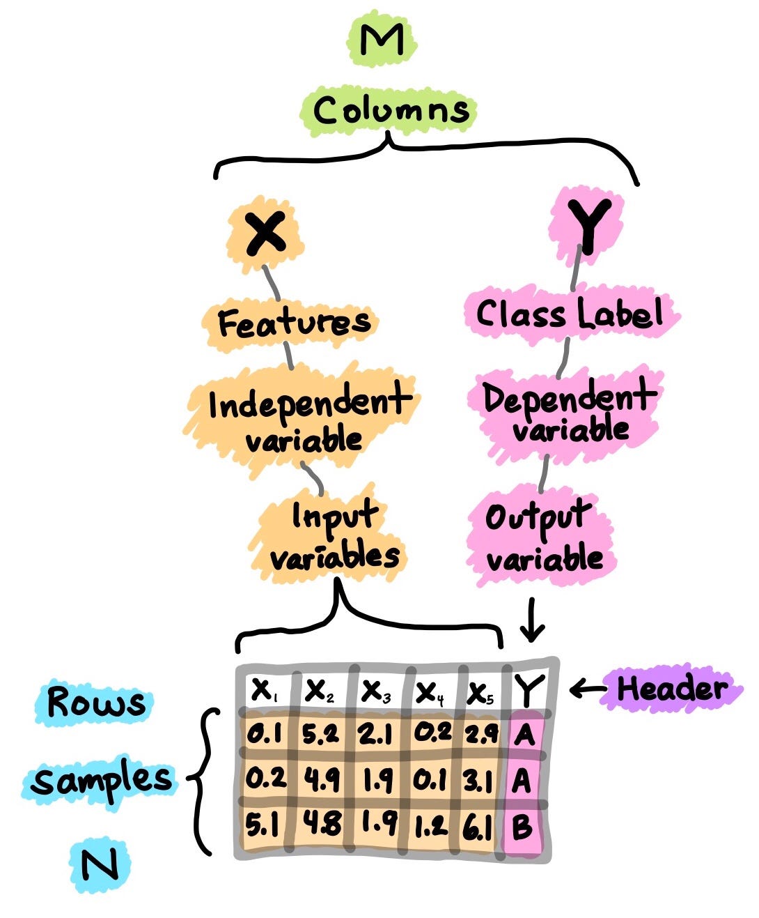
Cartoon illustration of a dataset. (Drawn by Chanin Nantasenamat)
It should be noted that a dataset that can be used for supervised learning (can perform either regression or classification) would contain both X and Y whereas a dataset that can be used for unsupervised learning will only have X.
Moreover, if Y contains quantitative values then the dataset (comprising of X and Y) can be used for regression tasks whereas if Y contains qualitative values then the dataset (comprising of X and Y) can be used for classification tasks.
Exploratory Data Analysis
Exploratory data analysis (EDA) is performed in order to gain a preliminary understanding and allow us to get acquainted with the dataset. In a typical data science project, one of the first things that I would do is “eyeballing the data” by performing EDA so as to gain a better understanding of the data.
Three major EDA approaches that I normally use includes:
Descriptive statistics — Mean, median, mode, standard deviation
Data visualisations — Heat maps (discerning feature intra-correlation), box plot (visualize group differences), scatter plots (visualize correlations between features), principal component analysis (visualize distribution of clusters presented in the dataset), etc.
Data shaping — Pivoting data, grouping data, filtering data, etc.
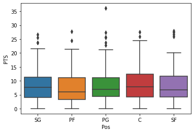
Example box plot of NBA player stats data. Plot obtained from the Jupyter notebook on Data Professor GitHub.
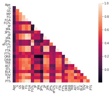
Example correlation heatmap of NBA player stats data. Plot obtained from the Jupyter notebook on Data Professor GitHub.
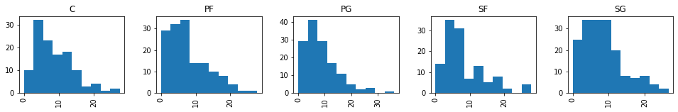
Example histogram plot of NBA player stats data. Plot obtained from the Jupyter notebook on Data Professor GitHub.
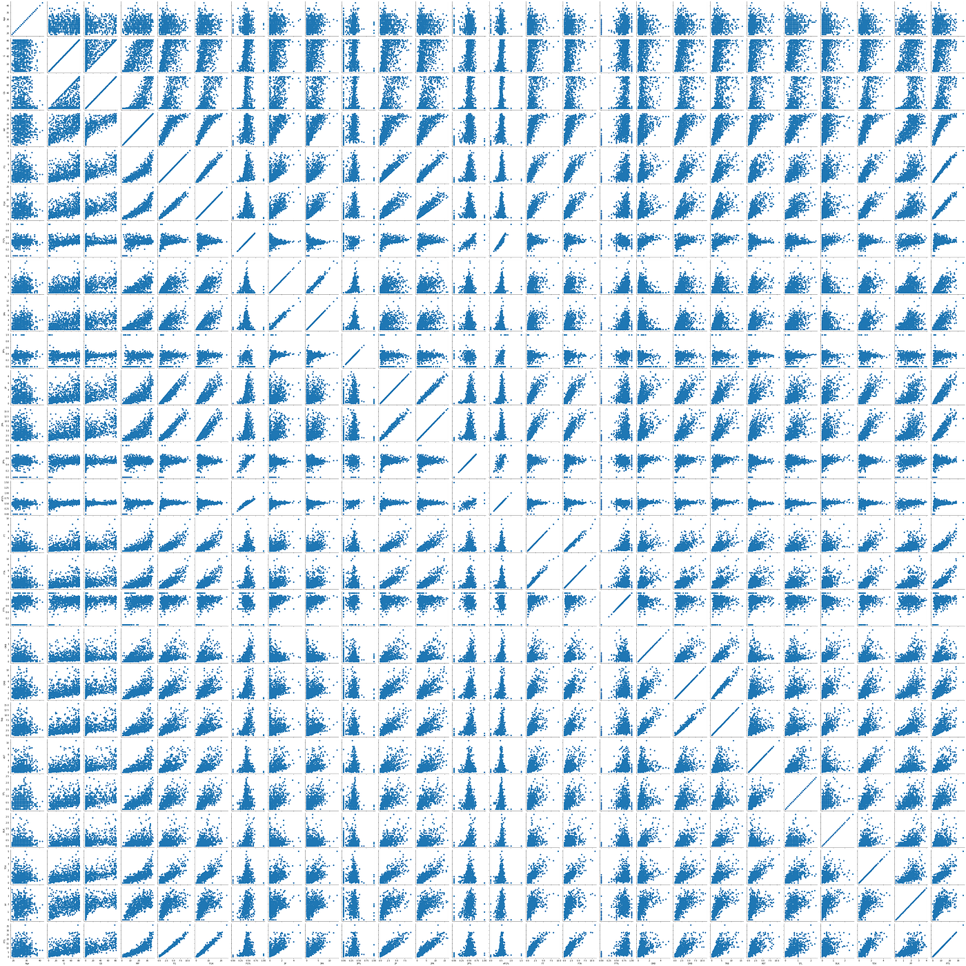
Example scatter plot of NBA player stats data. Plot obtained from the Jupyter notebook on Data Professor GitHub.
For more step-by-step tutorial on performing these exploratory data analysis in Python, please check out the video I made on the Data Professor YouTube channel.
Data Pre-Processing
Data pre-processing (also known as data cleaning, data wrangling or data munging) is the process by which the data is subjected to various checks and scrutiny in order to remedy issues of missing values, spelling errors, normalizing/standardizing values such that they are comparable, transforming data (e.g. logarithmic transformation), etc.
“Garbage in, Garbage out.”
As the above quote suggests, the quality of data is going to exert a big impact on the quality of the generated model. Therefore, to achieve the highest model quality, significant effort should be spent in the data pre-processing phase. It is said that data pre-processing could easily account for 80% of the time spent on data science projects while the actual model building phase and subsequent post-model analysis account for the remaining 20%.
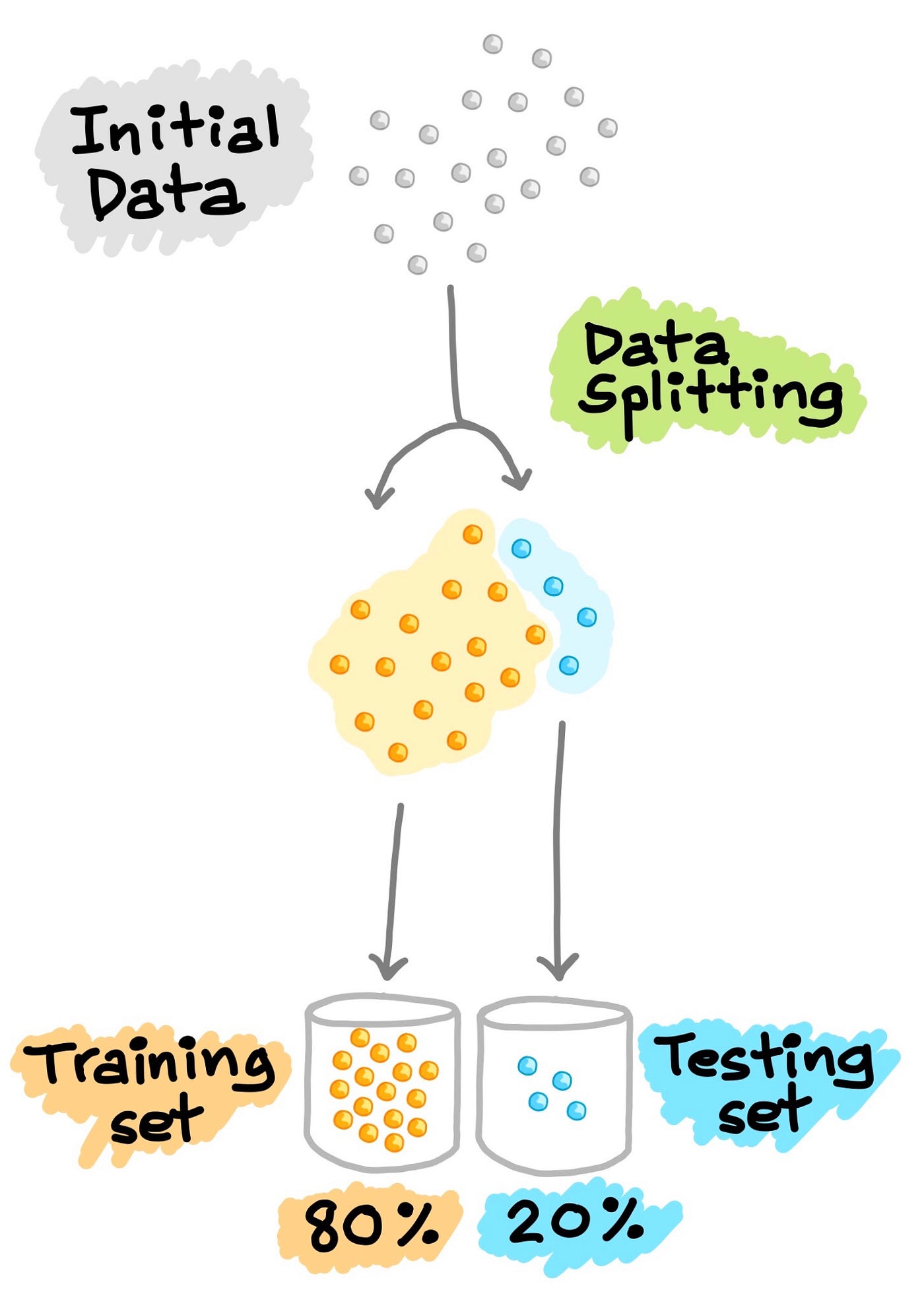
Data Splitting
Train-Test Split
In the development of machine learning models, it is desirable that the trained model perform well on new, unseen data. In order to simulate the new, unseen data, the available data is subjected to data splitting whereby it is split to 2 portions (sometimes referred to as the train-test split). Particularly, the first portion is the larger data subset that is used as the training set (such as accounting for 80% of the original data) and the second is normally a smaller subset and used as the testing set (the remaining 20% of the data). It should be noted that such data split is performed once.
Next, the training set is used to build a predictive model and such trained model is then applied on the testing set (i.e. serving as the new, unseen data) to make predictions. Selection of the best model is made on the basis of the model’s performance on the testing set and in efforts to obtain the best possible model, hyperparameter optimization may also be performed.
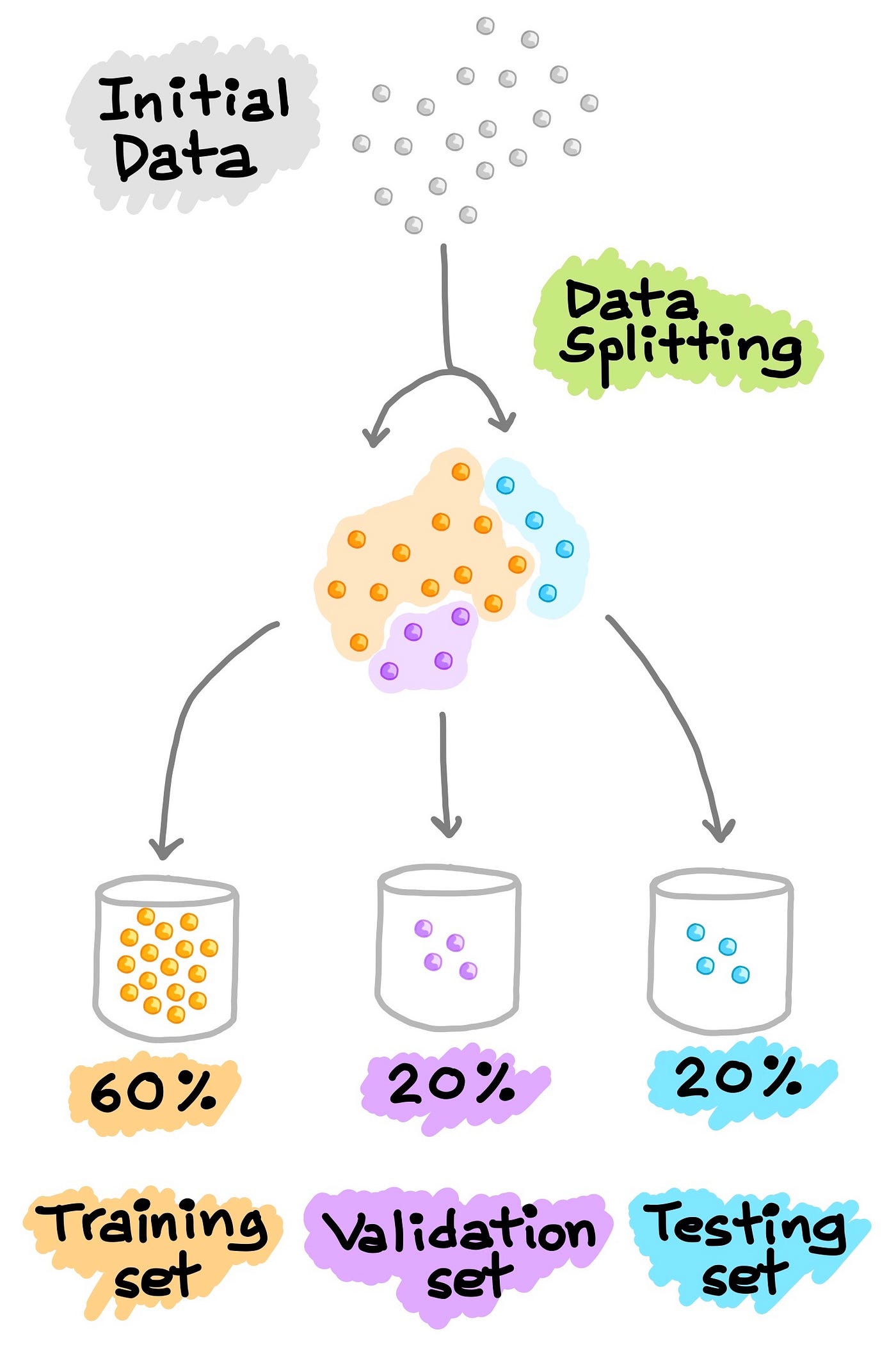
Train-Validation-Test Split
Another common approach for data splitting is to split the data to 3 portions: (1) training set, (2) validation set and (3) testing set. Similar to what was explained above, the training set is used to build a predictive model and is also evaluated on the validation set whereby predictions are made, model tuning can be made (e.g. hyperparameter optimization) and selection of the best performing model based on results of the validation set. As we can see, similar to what was performed above to the test set, here we do the same procedure on the validation set instead. Notice that the testing set is not involved in any of the model building and preparation. Thus, the testing set can truly act as the new, unseen data. A more in-depth treatment of this topic is provided by Google’s Machine Learning Crash Course.
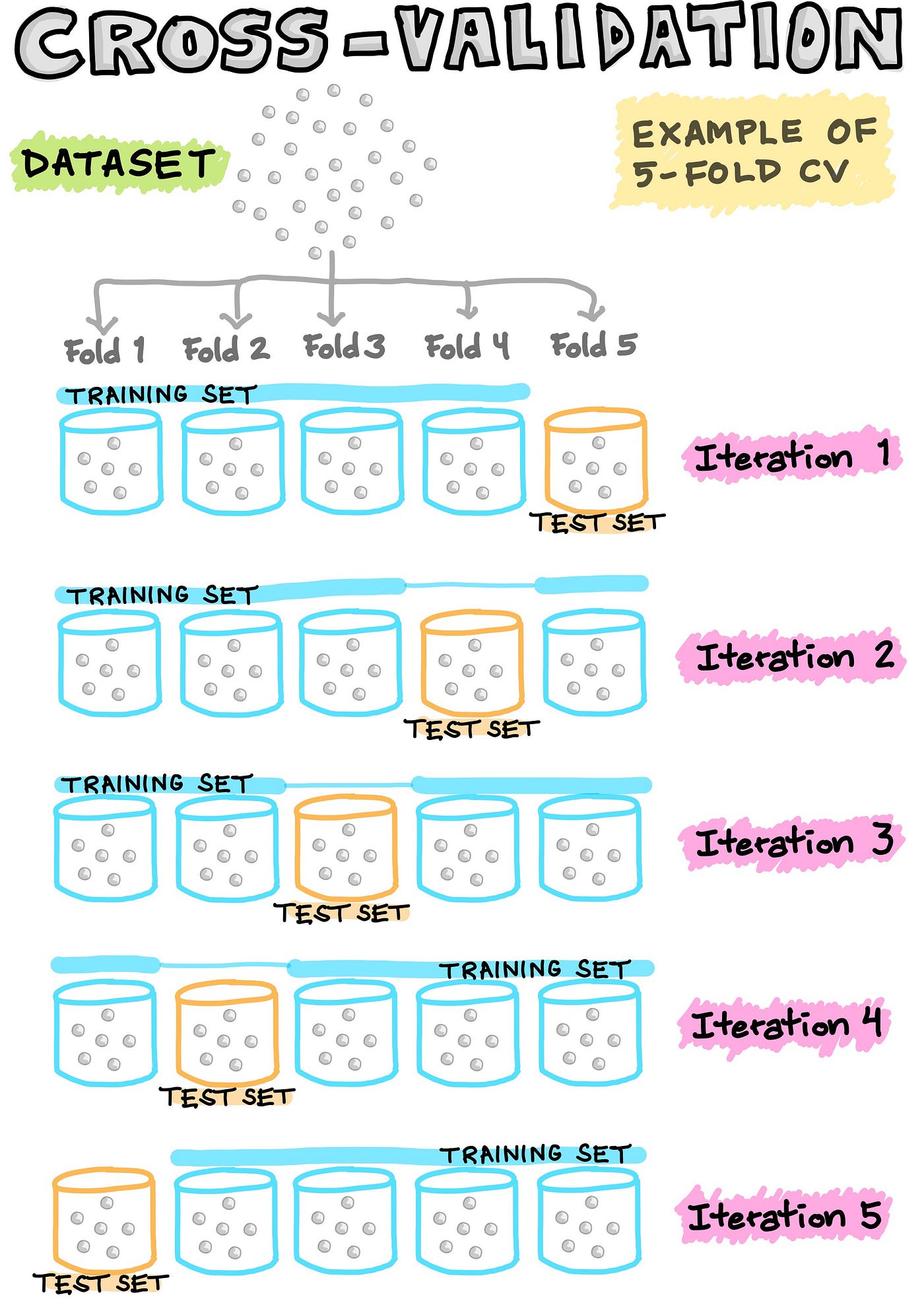
Cross-Validation
In order to make the most economical use of the available data, an N-fold cross-validation (CV) is normally used whereby the dataset is partitioned to N folds (i.e. commonly 5-fold or 10-fold CV are used). In such N-fold CV, one of the fold is left out as the testing data while the remaining folds are used as the training data for model building.
For example, in a 5-fold CV, 1 fold is left out and used as the testing data while the remaining 4 folds are pooled together and used as the training data for model building. The trained model is then applied on the aforementioned left-out fold (i.e. the test data). This process is carried out iteratively until all folds had a chance to be left out as the testing data. As a result, we will have built 5 models (i.e. where each of the 5 folds have been left out as the testing set) where each of the 5 models contain associated performance metrics (which we will discuss soon in the forthcoming section). Finally, the metric values are based on the average performance computed from the 5 models.
In situations when N is equal to the number of data samples, we call this leave-one-out cross-validation. In this type of CV, each data sample represents a fold. For example, if N is equal to 30 then there are 30 folds (1 sample per fold). As in any other N-fold CV, 1 fold is left out as the testing set while the remaining 29 folds are used to build the model. Next, the built model is applied to make prediction on the left-out fold. As before, this process is performed iteratively for a total of 30 times; and the average performance from the 30 models are computed and used as the CV performance metric.
Model Building
Now, comes the fun part where we finally get to use the meticulously prepared data for model building. Depending on the data type (qualitative or quantitative) of the target variable (commonly referred to as the Y variable) we are either going to be building a classification (if Y is qualitative) or regression (if Y is quantitative) model.
Learning Algorithms
Machine learning algorithms could be broadly categorised to one of three types:
Supervised learning — is a machine learning task that establishes the mathematical relationship between input X and output Y variables. Such X, Y pair constitutes the labeled data that are used for model building in an effort to learn how to predict the output from the input.
Unsupervised learning — is a machine learning task that makes use of only the input X variables. Such X variables are unlabeled data that the learning algorithm uses in modeling the inherent structure of the data.
Reinforcement learning — is a machine learning task that decides on the next course of action and it does this by learning through trial and error in an effort to maximize the reward.
Hyperparameter Optimization
Hyperparameters are essentially parameters of the machine learning algorithm that directly impacts the learning process and prediction performance. As there are no “one-size fits all” hyperparameter settings that will universally work for all datasets therefore one will need to perform hyperparameter optimization (also known as hyperparameter tuning or model tuning).
Let’s take random forest as an example. Two common hyperparameters that are typically subjected to optimization when using the randomForest R package includes the mtry and ntree parameters (this corresponds to n_estimators and max_features in RandomForestClassifier() and RandomForestRegressor() functions from the scikit-learn Python library). mtry (max_features) represents the number of variables that are randomly sampled as candidates at each split while ntree (n_estimators) represents the number of trees to grow.
Another popular machine learning algorithm is support vector machine. Hyperparameters to be optimized is the C and gamma parameters for the radial basis function (RBF) kernel (i.e. only the C parameter for the linear kernel; the C and exponential number for the polynomial kernel). The C parameter is a penalty term that limits overfitting while the gamma parameter controls the width of the RBF kernel. As mentioned above, tuning is typically performed so as to arrive at the optimal set of values to use for the hyperparameters and in spite of this there are research directed towards finding good starting values for the C and gamma parameters (Alvarsson et al. 2014).
Feature Selection
As the name implies, feature selection is literally the process of selecting a subset of features from an initially large volume of features. Aside from achieving highly accurate models, one of the most important aspect of machine learning model building is to obtain actionable insights and in order to achieve that it is important to be able to select a subset of important features from the vast number.
The task of feature selection in itself can constitute an entirely new area of research where intense efforts are geared toward devising novel algorithms and approaches. From amongst the plethora of available feature selection algorithms, some of the classical methods are based on simulated annealing and genetic algorithm. In addition to these, there are a large collection of approaches based on evolutionary algorithms (e.g. Particle Swarms Optimization, Ant Colony Optimization, etc.) and stochastic approaches (e.g. Monte Carlo).
Our own research group have also explored the use of Monte Carlo simulation for feature selection in a study of modeling the quantitative structure-activity relationship of aldose reductase inhibitors (Nantasenamat et al. 2014). We have also devised a novel feature selection approach based on combining two popular evolutionary algorithms namely genetic algorithm and particle swarm algorithm in our work entitled Genetic algorithm search space splicing particle swarm optimization as general-purpose optimizer (Li et al. 2013).
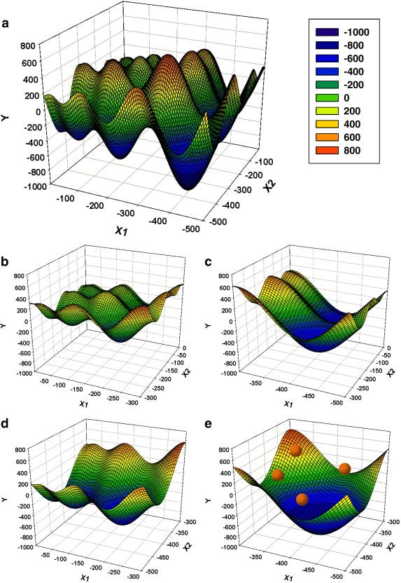
Schematic diagram of the principles of the genetic algorithm search space splicing particle swarms optimization (GA-SSS-PSO) approach as illustrated using the Schwefel function in 2 dimensions. “The original search space (a) x∈[–500,0] is spliced into sub-spaces at fixed interval of 2 at each dimension (a dimension equals an horizontal axis in the picture). This resulted in four subspaces (b–e) where the range of x at each dimension is half that of the original. Each string of GA encodes the indexes for one subspace. Then, GA heuristically selects a subspace (e) and PSO is initiated there (particles are shown as red dots). PSO searches for the global minimum of the subspaces and the best particle fitness is used as fitness of the GA string encoding the indexes for that subspace. Finally, GA undergoes evolution and selects a new subspace to explore. The whole process is repeated until satisfactory error level is reached.” (Reprinted from Chemometrics and Intelligent Laboratory Systems, Volume 128, Genetic algorithm search space splicing particle swarm optimization as general-purpose optimizer, Pages 153–159, Copyright (2013), with permission from Elsevier)
Machine Learning Tasks
Two common machine learning tasks in supervised learning includes classification and regression.
Classification
A trained classification model takes as input a set of variables (either quantitative or qualitative) and predicts the output class label (qualitative). The following figure hows three classes as indicated by the different colors and labels. Each small colored spheres represent a data sample whereby each sample
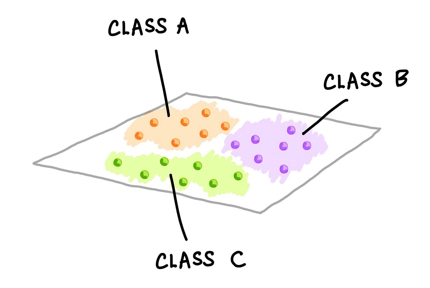
Schematic illustration of a multi-class classification problem. Three classes of data samples are shown in 2-dimensions. This drawing shows a hypothetical distribution of data samples. Such visualisation plot can be created by performing PCA analysis and displaying the first two principal components (PCs); alternatively a simple scatter plot of two variables can also be selected and visualized. (Drawn by Chanin Nantasenamat)
Example dataset
Take for example, the Penguins dataset (recently proposed as a replacement dataset for the heavily used Iris dataset) where we take as input quantitative (bill length, bill depth, flipper length and body mass)and qualitative (sex and island) features that uniquely describes the characteristics of penguins and classifying it as belonging to one of three species class label (Adelie, Chinstrap or Gentoo). The dataset is comprised of 344 rows and 8 columns. A prior analysis revealed that the dataset contains 333 complete cases where 19 missing values were presented in the 11 incomplete cases.

Artwork by @allison_horst
Performance metrics
How do we know when our model performs good or bad? The answer is to use performance metrics and some of the common ones for assessing the classification performance includes accuracy (Ac), sensitivity (Sn), specificity (Sp) and the Matthew’s correlation coefficient (MCC).
Equation for calculating the Accuracy.
Equation for calculating the Sensitivity.
Equation for calculating the Specificity.

Equation for calculating the Matthews Correlation Coefficient.
where TP, TN, FP and FN denote the instances of true positives, true negatives, false positives and false negatives, respectively. It should be noted that MCC ranges from −1 to 1 whereby an MCC of −1 indicates the worst possible prediction while a value of 1 indicates the best possible prediction scenario. Also, an MCC of 0 is indicative of random prediction.
Regression
In a nutshell, a trained regression model can be best summarised by the following simple equation:
Y=f(X)
where Y corresponds to the quantitative output variable, X refers to the input variables and f refers to the mapping function (obtained from the trained model) for computing the output values as a function of input features. The essence of the above equation for the regression example is that Y can be deduced if X is known. Once Y is calculated (we can also say ‘predicted’), a popular way to visualise the results is to make a simple scatter plot of the actual values versus the predicted values as shown below.
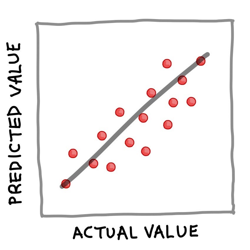
Simple scatter plot of actual versus predicted value. (Drawn by Chanin Nantasenamat)
Example dataset
The Boston Housing dataset is a popular example dataset typically used in data science tutorials. The dataset is comprised of 506 rows and 14 columns. For conciseness, shown below is the header (showing the names of variables) plus the first 4 rows of the dataset.
Of the 14 columns, the first 13 variables are used as input variables while the the median house price (medv) is used as the output variable. As can be seen all 14 variables contain quantitative values and thus suitable for regression analysis. I also made a step-by-step YouTube video showing how to build a linear regression model in Python.
In the video, I started by showing you how to read in the Boston Housing dataset, separating the data to X and Y matrices, perform 80/20 data split, build a linear regression model using the 80% subset and applying the trained model to make prediction on the 20% subset. Finally the performance metrics and scatter plot of the actual versus predicted medv values are shown.

Scatter plot of actual vs predicted medv values of the test set (20% subset). Plot taken from the Jupyter notebook on the Data Professor GitHub.
Performance metrics
Evaluation of the performance of regression models are performed to assess the degree at which a fitted model can accurately predict the values of input data.
Common metric for evaluating the performance of regression models is the coefficient of determination (R²).

As can be seen from the equation, R² is essentially 1 minus the ratio of the residual sum of squares to that of the total sum of squares. In simple terms, it can be said to represent the relative measure of explained variance. For example if R² = 0.6 then it means that the model could explain 60% of the variance (i.e. that is 60% of the data fits the regression model) whereas the unexplained variance accounted for the remaining 40%.
Additionally, the mean squared error (MSE) as well as the root mean squared error (RMSE) are also common measures of the residuals or error of prediction.

As can be seen from the above equation, the MSE is as the name implies easily computed by taking the mean of the squared error. Furthermore, a simple square root of the MSE yields the RMSE.
A Visual Explanation of the Classification Process
Now let’s take another look at the entire process of a classification model. Using the Penguins dataset as an example, we can see that penguins can be characterised by 4 quantitative features and 2 qualitative features, which are then used as input for training a classification model. In training the model, some of the issues that one would need to consider includes the following:
What machine learning algorithm to use?
What search space should be explored for hyperparameter optimization?
Which data splitting scheme to use? 80/20 split or 60/20/20 split? Or 10-fold CV?
Once the model has been trained, the resulting model can be used to make predictions on the class label (i.e. in our case the penguins species), which can be one of three penguins species: Adelie, Chinstrap or Gentoo.
Aside from performing only classification modeling, one could also perform principal component analysis (PCA), which will make use of only the X (independent) variables to discern the underlying structure of the data and in doing so would allow the visualisation of the inherent data clusters (shown below as a hypothetical plot where the clusters are color-coded according to the 3 penguins species).
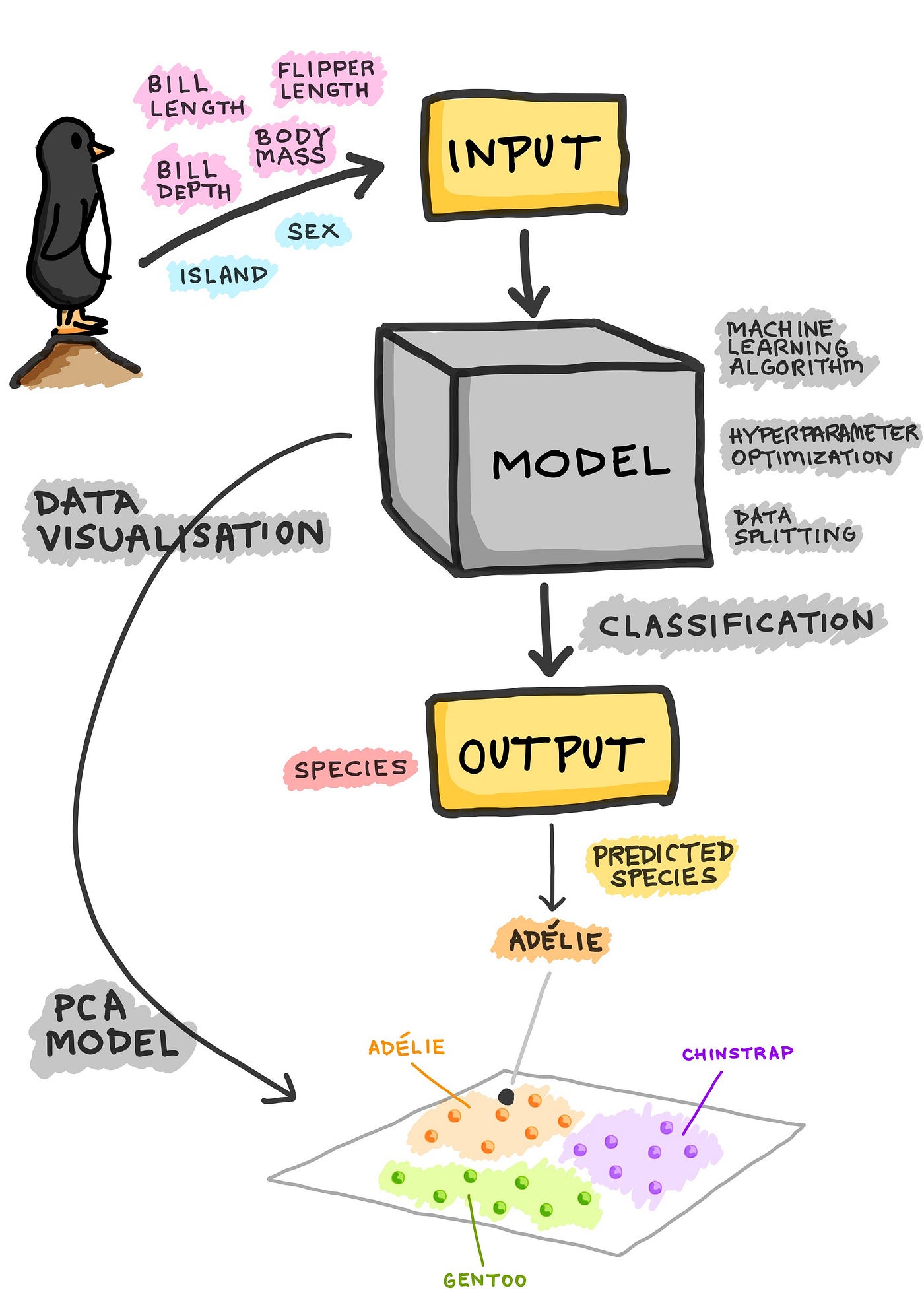
Schematic illustration of the process of building a classification model. (Drawn by Chanin Nantasenamat)
Cartoon infographic on building the machine learning model. Image drawn by Chanin Nantasenamat.