A while back I wrote a blog on How to Build a Machine Learning Model
(A Visual Guide to Learning Data Science) which takes you on a visual and conceptual journey on how a machine learning model is built. What the article did not show was how to implement the actual building of the model.

In this article, you will learn how to build your first machine learning model in Python. Particularly, you will be building regression models using traditional linear regression as well as other machine learning algorithms.

I’ve created the following YouTube video to serve as a supplement to this article, particularly it will get you up to speed on the concepts of machine learning model building as also covered in the first blog post mentioned above.

1. Your First Machine Learning Model

So what machine learning model are we building today? In this article, we are going to be building a regression model using the random forest algorithm on the solubility dataset.

After model building, we are going to apply the model to make predictions followed by model performance evaluation and data visualization of its results.

2. Dataset

2.1. Toy datasets

So which dataset are we going to use? The default answer may be to use a toy dataset as an example such as the Iris dataset (classification) or the Boston housing dataset (regression).

Although both are great examples to start out with, but typically most tutorials are not actually loading these data directly from an external source (i.e. such as from a CSV file) but instead are importing the data directly from a Python library such as the datasets sub-module of scikit-learn.

For instance, to load in the Iris dataset, one can use the following block of code:

from sklearn import datasets

iris = datasets.load_iris()
X = iris.data
y = iris.target

The benefit of using toy datasets is that they are super simple to use, simply import the data directly from the library in a format that can readily be used for model building. The downside of this convenience is that first-time learners may not actually see which functions are loading in the data, which ones are performing the actual pre-processing and which ones are building the model, etc.

2.2. Your own dataset

In this tutorial, we are going to take a practical approach where we will focus on building actual models that you can easily replicate. As we are going to be reading in the input data directly from a CSV file, thus you can easily replace the input data with your own data and repurpose the workflow described herein for your own data projects.

The dataset that we are using today is the solubility dataset. It is comprised of 1444 rows and 5 columns. Each row represents a unique molecule and each molecule is described by 4 molecular properties (the first 4 columns) while the last column is the target variable to be predicted. This target variable represents the solubility of a molecule, which is an important parameter of a therapeutic drug, as it helps a molecule travel inside the body to reach its target.

Below is the first few rows of the solubility dataset.

MolLogP,MolWt,NumRotatableBonds,AromaticProportion,logS
2.5954000000000006,167.85,0.0,0.0,-2.18
2.376500000000001,133.405,0.0,0.0,-2.0
2.5938,167.85,1.0,0.0,-1.74
2.0289,133.405,1.0,0.0,-1.48
2.9189,187.37500000000003,1.0,0.0,-3.04

2.2.1. Loading data

The full solubility dataset is available on the Data Professor GitHub at the following link: Download Solubility dataset.

To be usable for any data science project, data contents from CSV files can be read into the Python environment using the Pandas library. I’ll show you how in the example below:

import pandas as pd

df = pd.read_csv('data.csv')

The first line imports the pandas library as a short acronym form referred to as pd (for ease of typing). From pd, we’re going to use it’s read_csv() function and thus we type in pd.read_csv(). By typing pd in front, we therefore know from which library the read_csv() function belongs to.

The input argument inside the read_csv() function is the CSV file name which in our example above is 'data.csv’. Here, we assign the data contents from the CSV file to a variable called df.

In this tutorial, we’re going to use the solubility dataset (available at https://raw.githubusercontent.com/dataprofessor/data/master/delaney_solubility_with_descriptors.csv). Thus, we would load in the data using the following code:

import pandas as pd

df = pd.read_csv('https://raw.githubusercontent.com/dataprofessor/data/master/delaney_solubility_with_descriptors.csv')

2.2.2. Data processing

Now that we have the data as a dataframe in the df variable, we will now need to prepare it to be in a suitable format to be used by the scikit-learn library because the df is not yet usable by the library.

How do we do that? We will need to separate them into 2 variables X and y.

The first 4 columns except for the last column will be assigned to the X variable while the last column will be assigned to the y variable.

2.2.2.1. Assigning variables to X

To assign the first 4 columns to the X variable, we will use the following lines of code:

X = df.drop(['logS'], axis=1)

As we can see, we did this by dropping or removing the last column (logS).

2.2.2.2. Assigning variable to y

To assign the last column to the y variable, we simple select the last column and assign it to the y variable as follows:

y = df.iloc[:,-1]

As we can see, we did this by explicitly selecting the last column. Two alternative approaches can also be done to get the same results where the first approach is as follows:

y = df["logS"]

And the second approach is as follows:

y = df.logS

Choose 1 of the above of your choice and continue to the next step.

3. Data splitting

Data splitting allows unbiased evaluation of the model’s performance on fresh data that was not previously seen by the model. Particularly, if the full dataset is split into a training set and a testing set using an 80/20 split ratio then the model could be built using the 80% data subset (i.e. which we can call the training set) and subsequently evaluated on the 20% data subset (i.e. which we can call the test set). In addition to applying the trained model on the test set, we can also apply the trained model on the training set (i.e. data used to construct the model in the first place).

Subsequent comparison of the model performance of both data splits (i.e. training set and test set) will allow us to evaluate whether the model is underfitting or overfitting. Underfitting typically occurs whether both performance of training set and test set are poor whereas in overfitting the test set is significantly underperforming when compared to the training set.

To perform the data splitting, the scikit-learn library has the train_test_split() function that allows us to do this. An example of using this function to split the dataset into the training set and test set is shown below:

from sklearn.model_selection import train_test_split

X_train, X_test, y_train, y_test = train_test_split(
    X, y, test_size=0.2, random_state=42)

In the above code, the first line imports the train_test_split() function from sklearn.model_selection sub-module. As we can see, the input argument consists of the X and y input data, the test set size is specified to 0.2 (i.e. 20% of the data will go to the test set whereas the remaining 80% to the training set) and the random seed number is set to 42.

From the above code, we can see that we had simultaneously created 4 variables consisting of the separated X and y variables for the training set (X_train and y_train) and test set (X_test and y_test).

Now we are ready to use these 4 variables for model building.

4. Model building

Here comes the fun part! We’re now going to build some regression models.

4.1. Linear regression

4.1.1. Model building

Let’s start with the traditional linear regression.

from sklearn.linear_model import LinearRegression

lr = LinearRegression()
lr.fit(X_train, y_train)

The first line imports the LinearRegression() function from the sklearn.linear_model sub-module. Next, the LinearRegression() function is assigned to the lr variable and the .fit() function performs the actual model training on the input data X_train and y_train.

Now that the model is built, we’re going to apply it to make predictions on the training set and test set as follows:

y_lr_train_pred = lr.predict(X_train)
y_lr_test_pred = lr.predict(X_test)

As we can see in the above code, the model (lr) is applied to make predictions via the lr.predict() function on the training set and test set.

4.1.2. Model performance

We’re now going to calculate the performance metrics so that we will be able to determine the model performance.

from sklearn.metrics import mean_squared_error, r2_score

lr_train_mse = mean_squared_error(y_train, y_lr_train_pred)
lr_train_r2 = r2_score(y_train, y_lr_train_pred)

lr_test_mse = mean_squared_error(y_test, y_lr_test_pred)
lr_test_r2 = r2_score(y_test, y_lr_test_pred)

In the above code, we import the mean_squared_error and r2_score functions from the sklearn.metrics sub-module to compute the performance metrics. The input arguments for both functions are the actual Y values (y) and the predicted Y values (y_lr_train_pred and y_lr_test_pred).

Let’s talk about the naming convention used here, we assign the function to self-explanatory variables explicitly telling the what the variable contains. For example, lr_train_mse and lr_train_r2 explicitly tells that the variables contain the performance metrics MSE and R2 for models build using linear regression on the training set. The advantage of using this naming convention is that performance metrics of any future models built using a different machine learning algorithm could be easily identified by its variable names. For example, we could use rf_train_mse to denote the MSE of the training set for a model built using random forest.

The performance metrics can be displayed by simply printing the variables. For instance, to print out the MSE for the training set:

print(lr_train_mse)

which gives 1.0139894491573003.

To see the results for the other 3 metrics, we could print them one by one as well but that would be a bit repetitive.

Another way is to produce a tidy display of the 4 metrics as follows:

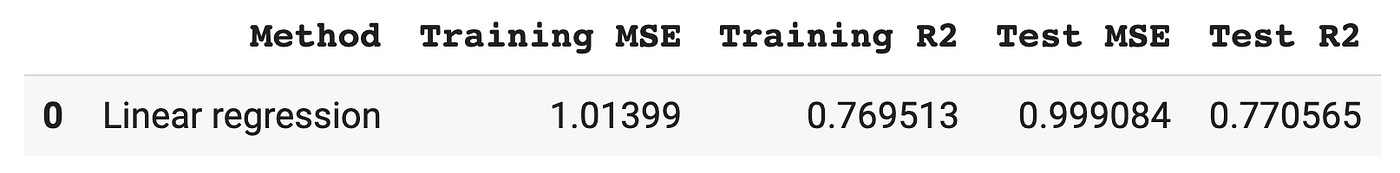
lr_results = pd.DataFrame(['Linear regression',lr_train_mse, lr_train_r2, lr_test_mse, lr_test_r2]).transpose()

lr_results.columns = ['Method','Training MSE','Training R2','Test MSE','Test R2']

which produces the following dataframe:

4.2. Random forest

Random forest (RF) is an ensemble learning method whereby it combine the predictions of several decision trees. A great thing about RF is its built-in feature importance (i.e. the Gini index values that it produces for constructed models).

4.2.1. Model building

Let’s now build an RF model using the following code:

from sklearn.ensemble import RandomForestRegressor

rf = RandomForestRegressor(max_depth=2, random_state=42)
rf.fit(X_train, y_train)

In the above code, the first line imports the RandomForestRegressor function (i.e. can also be called a regressor) from the sklearn.ensemble sub-module. It should be noted here that RandomForestRegressor is the regression version (i.e. this is used for when the Y variable comprises of numerical values) while its sister version is the RandomForestClassifier, which is the classification version (i.e. this is used for when the Y variable contains categorical values).

In this example, we are setting the max_depth parameter to be 2 and random seed number (via random_state) to be 42. Finally, the model is trained using the rf.fit() function where we set X_train and y_train as the input data.

We’re now going to apply the constructed model to make predictions on the training set and test set as follows:

y_rf_train_pred = rf.predict(X_train)
y_rf_test_pred = rf.predict(X_test)

In a similar fashion to that used in the lr model, the rf model is also applied to make predictions via the rf.predict() function on the training set and test set.

4.2.2. Model performance

Let’s now calculate the performance metrics for the constructed random forest model as follows:

from sklearn.metrics import mean_squared_error, r2_score

rf_train_mse = mean_squared_error(y_train, y_rf_train_pred)
rf_train_r2 = r2_score(y_train, y_rf_train_pred)

rf_test_mse = mean_squared_error(y_test, y_rf_test_pred)
rf_test_r2 = r2_score(y_test, y_rf_test_pred)

To consolidate the results, we use the following code:

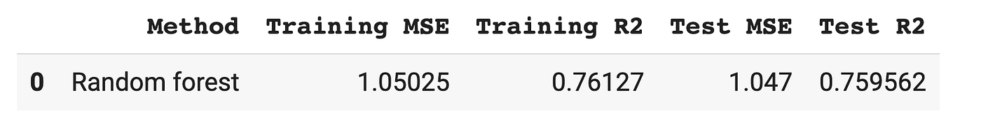
rf_results = pd.DataFrame(['Random forest',rf_train_mse, rf_train_r2, rf_test_mse, rf_test_r2]).transpose()

rf_results.columns = ['Method','Training MSE','Training R2','Test MSE','Test R2']

which produces:

4.3. Other machine learning algorithms

To build models using other machine learning algorithms (aside from sklearn.ensemble.RandomForestRegressor that we had used above), we need only decide on which algorithms to use from the available regressors (i.e. since the dataset’s Y variable contain categorical values).

4.3.1. List of regressors

Let’s take a look at some example regressors that we can choose from:

• sklearn.linear_model.Ridge

• sklearn.linear_model.SGDRegressor

• sklearn.ensemble.ExtraTreesRegressor

• sklearn.ensemble.GradientBoostingRegressor

• sklearn.neighbors.KNeighborsRegressor

• sklearn.neural_network.MLPRegressor

• sklearn.tree.DecisionTreeRegressor

• sklearn.tree.ExtraTreeRegressor

• sklearn.svm.LinearSVR

• sklearn.svm.SVR

For a more extensive list of regressors, please refer to the Scikit-learn’s API Reference.

4.3.2. Using a regressor

Let’s say that we would like to use sklearn.tree.ExtraTreeRegressor we would use as follows:

from sklearn.tree import ExtraTreeRegressor

et = ExtraTreeRegressor(random_state=42)
et.fit(X_train, y_train)

Note how we import the regressor function for sklearn.tree.ExtraTreeRegressor as follows:
from sklearn.tree import ExtraTreeRegressor

Afterwards, the regressor function is then assigned to a variable (i.e. et in this example) and subjected to model training via the .fit() function as in et.fit().

4.4. Combining the Results

Let’s recall that the model performance metrics that we had previously generated above for linear regression and random forest models are stored in the lr_results and rf_results variables.

As both variables are dataframes, we are going to combine them using the pd.concat() function as shown below:

pd.concat([lr_results, rf_results])

This produces the following dataframe:

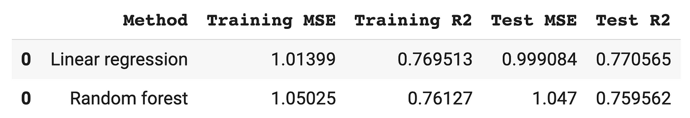
It should be noted that performance metrics for additional learning methods could also be added by appending to the list [lr_results, rf_results].

For example, svm_results could be added to the list, which would then become [lr_results, rf_results, svm_results].

5. Data visualization of prediction results

Let’s now visualize the relationship of the actual Y values with their predicted Y values that is the experimental logS versus the predicted logS values.

import matplotlib.pyplot as plt
import numpy as np

plt.figure(figsize=(5,5))
plt.scatter(x=y_train, y=y_lr_train_pred, c="#7CAE00", alpha=0.3)

z = np.polyfit(y_train, y_lr_train_pred, 1)
p = np.poly1d(z)

plt.plot(y_train,p(y_train),"#F8766D")
plt.ylabel('Predicted LogS')
plt.xlabel('Experimental LogS')

As shown above, we’re going to use the Matplotlib library for making the scatter plot while Numpy is used for generating the trend line of the data. Here, we’re setting the figure size to be 5 × 5 via the figsize parameter of the plt.figure() function.

The plt.scatter() function is used to create the scatter plot where y_train and y_lr_train_pred (i.e. training set predictions made by linear regression) are used as input data. The color is set to be green using the HTML color code (Hex code) of #7CAE00.

A trend line to the plot via the np.polyfit() function and is displayed via plt.plot() function as shown above. Finally, the X-axis and Y-axis labels are added via the plt.xlabel() and plt.ylabel() functions, respectively.

The rendered scatter plot is shown to the left.

What’s Next?

Congratulations on building your first machine learning model!

What’s next, you may ask. The answer is quite simple, build more models! Tweak the parameters, try out new algorithms, tinker with the addition of new features to the machine learning pipeline and most importantly of all don’t be fearful of making mistakes. In fact, the fastest route to turbo charging your learning is to fail often, get back up and try again. Learning is about enjoying the process and if you persist long enough, you’ll gain more confident in your path of becoming a data professional whether it be a data science, data analyst or data engineer. But most importantly of all, as I always like to say:

Created (with license) using the image by aqrstudio from envato elements.