- Data Professor
- Posts
- How to Tune Hyperparameters of Machine Learning Models
How to Tune Hyperparameters of Machine Learning Models
A Step-by-Step Tutorial using Scikit-learn
Chanin Nantasenamat
June 07, 2021

Often times you’re using default parameters for building machine learning models. In just a few blocks of code you can search for the best hyperparameters for your machine learning models. Why? Because the optimal set of hyperparameters can go a long way to significantly boost the performance of your models.
In this article, you will learn how to perform hyperparameter tuning of the random forest model in Python using the scikit-learn library.
Note: This article was inspired by a YouTube video I made some time ago (Hyperparameter Tuning of Machine Learning Model in Python).
1. Hyperparameters
In applied machine learning, tuning the machine learning model’s hyperparameters represent a lucrative opportunity to achieve the best performance as possible.
1.1. Parameters vs Hyperparameters
Let’s now define what are hyperparameters, but before doing that let’s consider the difference between a parameter and a hyperparameter.
A parameter can be considered to be intrinsic or internal to the model and can be obtained after the model has learned from the data. Examples of parameters are regression coefficients in linear regression, support vectors in support vector machines and weights in neural networks.
A hyperparameter can be considered to be extrinsic or external to the model and can be set arbitrarily by the practitioner. Examples of hyperparameters include the k in k-nearest neighbors, number of trees and maximum number of features in random forest, learning rate and momentum in neural networks, the C and gamma parameters in support vector machines.
1.2. Hyperparameter tuning
As there are no universal best hyperparameters to use for any given problem, hyperparameters are typically set to default values. However, the optimal set of hyperparameters can be obtained from manual empirical (trial-and-error) hyperparameter search or in an automated fashion via the use of optimization algorithm to maximize the fitness function.
Two common hyperparameter tuning methods include grid search and random search. As the name implies, a grid search entails the creation of a grid of possible hyperparameter values whereby models are iteratively built for all of these hyperparameter combinations in a brute force manner. In a random search, not all hyperparameter combinations are used, but instead each iteration makes use of a random hyperparameter combination.
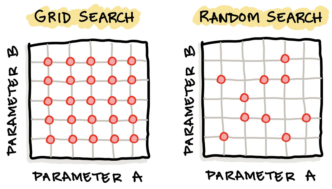
Schematic illustration comparing the 2 common hyperparameter tuning approach: (1) grid search with (2) random search. Image drawn by the Author.
Additionally, a stochastic optimization approach may also be applied for hyperparameter tuning which will automatically navigate the hyperparameter space in an algorithmic manner as a function of the loss function (i.e. the performance metrics) in order to monitor the model performance.
In this tutorial, we will be using the grid search approach.
2. Dataset
Today, we’re not going to use the Iris dataset nor the Penguins dataset but instead we’re going to generate our very own synthetic dataset. However, if you would like to follow along and substitute with your own dataset that would be great!
2.1. Generating the Synthetic Dataset
from sklearn.datasets import make_classification

X, Y = make_classification(n_samples=200, n_classes=2, n_features=10, n_redundant=0, random_state=1)
2.2. Examine Dataset Dimension
Let’s now examine the dimension of the dataset
X.shape, Y.shapewhich should give the following output:
((200, 10), (200,)) where (200, 10) is the dimension of the X variable and here we can see that there are 200 rows and 10 columns. As for (200,), this is the dimension of the Y variable and this indicates that there are 200 rows and 1 column (no numerical value shown).
3. Data Splitting
from sklearn.model_selection import train_test_split

X_train, X_test, Y_train, Y_test = train_test_split(X, Y, test_size=0.2)
3.1. Examining the Dimension of Training Set
Let’s now examine the dimension of the training set (the 80% subset).
X_train.shape, Y_train.shapewhich should give the following output:
((160, 10), (160,)) where (160, 10) is the dimension of the X variable and here we can see that there are 160 rows and 10 columns. As for (160,), this is the dimension of the Y variable and this indicates that there are 200 rows and 1 column (no numerical value shown).
3.2. Examining the Dimension of Training Set
Let’s now examine the dimension of the testing set (the 20% subset).
X_test.shape, Y_test.shapewhich should give the following output:
((40, 10), (40,)) where (40, 10) is the dimension of the X variable and here we can see that there are 40 rows and 10 columns. As for (40,), this is the dimension of the Y variable and this indicates that there are 40 rows and 1 column (no numerical value shown).
4. Building a Baseline Random Forest Model
Here, we will first start by building a baseline random forest model that will serve as a baseline for comparative purpose with the model using the optimal set of hyperparameters.
For the baseline model, we will set an arbitrary number for the 2 hyperparameters (e.g. n_estimators and max_features) that we will also use in the next section for hyperparameter tuning.
4.1. Instantiating the Random Forest Model
We first start by importing the necessary libraries and assigning the random forest classifier to the rf variable.
from sklearn.ensemble import RandomForestClassifier
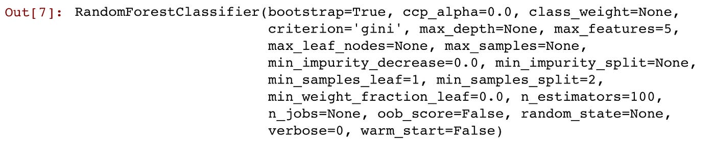
rf = RandomForestClassifier(max_features=5, n_estimators=100)4.2. Training the Random Forest Model
Now, we will be applying the random forest classifier to build the classification model using the rf.fit() function on the training data (e.g. X_train and Y_train).
rf.fit(X_train, Y_train)
Y_pred = rf.predict(X_test)
After the model has been trained, the following output appears:
Afterwards, we can apply the trained model (rf) for making predictions. In the example code above we apply the model to predict the training set (X_test) and assign the predicted Y values to the Y_pred variable.
4.3. Evaluating the Model Performance
Let’s now evaluate the model performance. Here, we’re calculating 3 performance metrics consisting of Accuracy, Matthews Correlation Coefficient (MCC) and the Area Under the Receiver Operating Characteristic Curve (ROC AUC).
from sklearn.metrics import accuracy_score, matthews_corrcoef, roc_auc_score

ac = accuracy_score(Y_pred, Y_test)
mcc = matthews_corrcoef(Y_pred, Y_test)
roc_auc = roc_auc_score(Y_pred, Y_test)
5. Hyperparameter Tuning
Now we will be performing the tuning of hyperparameters of the random forest model. The 2 hyperparameters that we will tune includes max_features and the n_estimators.
5.1. The Code
It should be noted that some of the code shown below were adapted from scikit-learn.
from sklearn.model_selection import GridSearchCV
import numpy as np

max_features_range = np.arange(1,6,1)
n_estimators_range = np.arange(10,210,10)
param_grid = dict(max_features=max_features_range, n_estimators=n_estimators_range)

rf = RandomForestClassifier()

grid = GridSearchCV(estimator=rf, param_grid=param_grid, scoring='roc_auc', cv=5)

grid.fit(X_train, Y_train)

print("The best parameters are %s with a score of %0.2f"
      % (grid.best_params_, grid.best_score_))
5.2. Code Explanation
Firstly, we will import the necessary libraries.
The GridSearchCV() function from scikit-learn will be used to perform the hyperparameter tuning. Particularly, is should be noted that the GridSearchCV() function can perform the typical functions of a classifier such as fit, score and predict as well as predict_proba, decision_function, transform and inverse_transform.
Secondly, we define variables that are necessary input to the GridSearchCV() function and this included the range values of the 2 hyperparameters (max_features_range and n_estimators_range), which is then assigned as a dictionary to the param_grid variable.
Finally, the best parameters (grid.best_params_) along with their corresponding metric (grid.best_score_) are printed out.
5.3. Performance Metrics
The default performance metric for GridSearchCV() is accuracy and in this example we’re going to use ROC AUC.
Just in case, you’re wondering what other performance metrics can be used, run the following command to find out:
import sklearn
sorted(sklearn.metrics.SCORERS.keys())
This prints the following supported performance metrics:
['accuracy',
 'adjusted_mutual_info_score',
 'adjusted_rand_score',
 'average_precision',
 'balanced_accuracy',
 'completeness_score',
 'explained_variance',
 'f1',
 'f1_macro',
 'f1_micro',
 'f1_samples',
 'f1_weighted',
 'fowlkes_mallows_score',
 'homogeneity_score',
 'jaccard',
 'jaccard_macro',
 'jaccard_micro',
 'jaccard_samples',
 'jaccard_weighted',
 'max_error',
 'mutual_info_score',
 'neg_brier_score',
 'neg_log_loss',
 'neg_mean_absolute_error',
 'neg_mean_gamma_deviance',
 'neg_mean_poisson_deviance',
 'neg_mean_squared_error',
 'neg_mean_squared_log_error',
 'neg_median_absolute_error',
 'neg_root_mean_squared_error',
 'normalized_mutual_info_score',
 'precision',
 'precision_macro',
 'precision_micro',
 'precision_samples',
 'precision_weighted',
 'r2',
 'recall',
 'recall_macro',
 'recall_micro',
 'recall_samples',
 'recall_weighted',
 'roc_auc',
 'roc_auc_ovo',
 'roc_auc_ovo_weighted',
 'roc_auc_ovr',
 'roc_auc_ovr_weighted',
 'v_measure_score']
Thus, in this example we are going to use ROC AUC and thus set the input argument scoring = 'roc_auc' inside the GridSearchCV() function.
5.4. Results from Hyperparameter Tuning
Lines 14–15 from the code in section 5.1 prints the performance metrics as shown below:

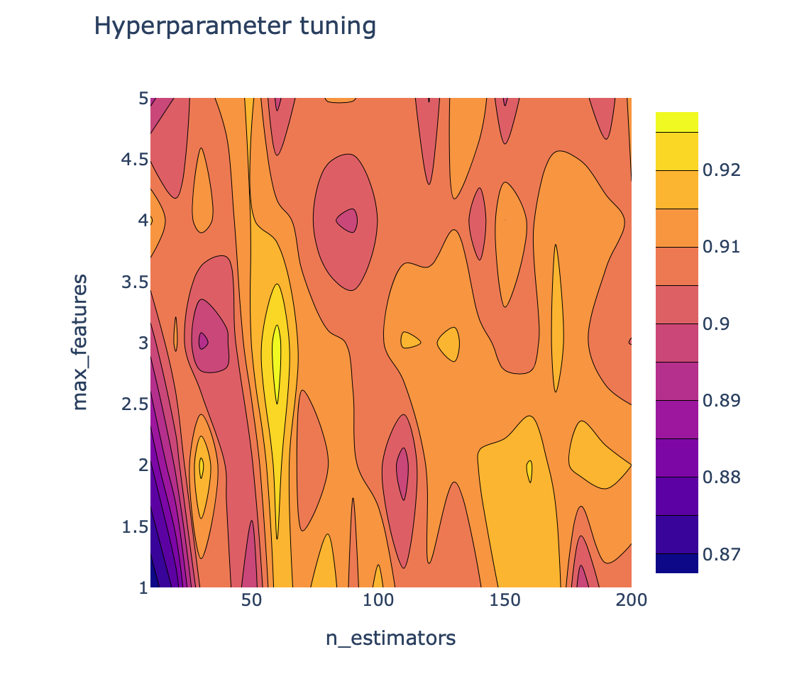
which indicated that the optimal or best set of hyperparameters has a max_features of 3 and an n_estimators of 60 with an ROC AUC score of 0.93.
6. Data Visualization of Tuned Hyperparameters
Let’s first start by taking a look at the underlying data where we will later use it for data visualization. Results from hyperpameter tuning has been written out to grid.cv_results_ whose contents are shown below as a dictionary data type shown below.
Screenshot of the contents of grid.cv_results_.
6.1. Preparing the DataFrame
Now, we’re going to selectively extract some data from grid.cv_results_ to create a dataframe containing the 2 hyperparameter combinations along with their corresponding performance metric, which in this case is the ROC AUC. Particularly, the following code block allows the combining of 2 hyperparameters (params) and the performance metric (mean_test_score).
import pandas as pd

grid_results = pd.concat([pd.DataFrame(grid.cv_results_["params"]),
                          pd.DataFrame(grid.cv_results_["mean_test_score"],
                          columns=["ROC_AUC"])],
                          axis=1)

grid_results
The output is the following dataframe with the 3 columns consisting of max_features, n_estimators and ROC_AUC.
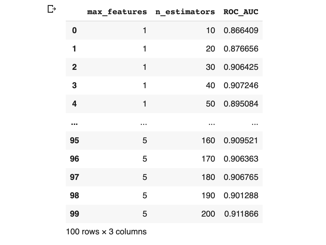
Screenshot of the output of the concatenated dataframe containing the hyperparameter combinations and their corresponding performance metric value.
6.2. Reshaping the DataFrame
6.2.1. Grouping the columns
In order to visualize the above dataframe as a contour plot (i.e. either 2D or 3D version), we will first need to reshape the data structure.
grid_contour = grid_results.groupby(['max_features','n_estimators']).mean()
grid_contour
In the above code, we’re using the groupby() function from the pandas library to literally group the dataframe according to 2 columns (max_features and n_estimators) whereby the contents of the first column (max_features) are merged.
6.2.2. Pivoting the data
Data is reshaped by pivoting the data into an m ⨯ n matrix where rows and columns correspond to the max_features and n_estimators, respectively.
grid_reset = grid_contour.reset_index()
grid_reset.columns = ['max_features', 'n_estimators', 'ROC_AUC']
grid_pivot = grid_reset.pivot('max_features', 'n_estimators')
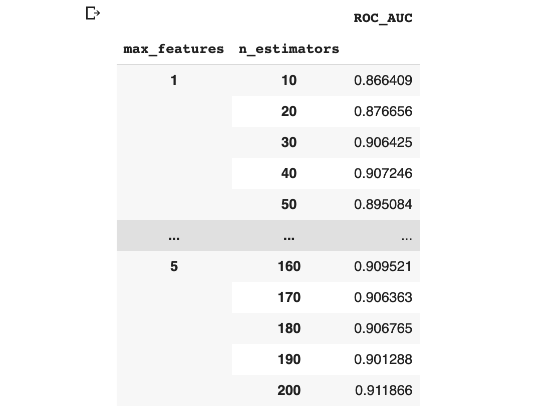
grid_pivotThe above code block produces the following reshaped dataframe.
Screenshot of the reshaped dataframe that is ready for making a contour plot.
Finally, we assign the reshaped data to the respective x, y and z variables that will then be used for making the contour plot.
x = grid_pivot.columns.levels[1].values
y = grid_pivot.index.values
z = grid_pivot.values
6.3. Making the 2D Contour Plot
Now, comes the fun part, we will be visualizing the landscape of the 2 hyperparameters that we are tuning and their influence on the ROC AUC score by making the 2D contour plot using Plotly. The aforementioned x, y and z variables are used as the input data.
import plotly.graph_objects as go

# X and Y axes labels
layout = go.Layout(
            xaxis=go.layout.XAxis(
              title=go.layout.xaxis.Title(
              text='n_estimators')
             ),
             yaxis=go.layout.YAxis(
              title=go.layout.yaxis.Title(
              text='max_features')
            ) )

fig = go.Figure(data = [go.Contour(z=z, x=x, y=y)], layout=layout )

fig.update_layout(title='Hyperparameter tuning', autosize=False,
                  width=500, height=500,
                  margin=dict(l=65, r=50, b=65, t=90))

fig.show()
The above code block generates the following 2D contour plot.
6.4. Making the 3D Contour Plot
Here, we’re going to use Plotly for creating an interactive 3D contour plot using the x, y and z variables as the input data.
import plotly.graph_objects as go

fig = go.Figure(data= [go.Surface(z=z, y=y, x=x)], layout=layout )

fig.update_layout(title='Hyperparameter tuning',
                  scene = dict(
                    xaxis_title='n_estimators',
                    yaxis_title='max_features',
                    zaxis_title='ROC_AUC'),
                  autosize=False,
                  width=800, height=800,
                  margin=dict(l=65, r=50, b=65, t=90))

fig.show()
The above code block generates the following 3D contour plot.
Screenshot of the 3D contour plot of the 2 hyperparameters against the performance metric ROC AUC.
Conclusion
Congratulations! You have just performed hyperparameter tuning as well as create data visualizations to go along with it. Hopefully, you’ll be able to boost your model performance as compare to those achieved by the default values.
What’s next? In this tutorial, you have explored the tuning of 2 hyperparameters but that’s not all. There are several other hyperparameters that you could tune for random forest model. You can check out the API from scikit-learn for a list of hyperparameters to try out.
Or perhaps you can try tuning hyperparameters for other machine learning algorithms by using the code described in this article as a starting template.
Let me know in the comments, what fun projects are you working on!
Created (with license) using the image by BoykoPictures from envato elements.