- Data Professor
- Posts
- How to Use Machine Learning for Drug Discovery
How to Use Machine Learning for Drug Discovery
A Step-by-Step Practical Bioinformatics Tutorial
Chanin Nantasenamat
June 07, 2020

1. Introduction
We have probably seen the application of machine learning in one form or another. For instance, machine learning have been used together with computer vision in self-driving cars and self-checkout convenience stores, in retail for market basket analysis (i.e. finding products that are usually purchased together), in entertainment for recommendation systems and the list goes on.
This represents the first article of the Bioinformatics Tutorial series (Thanks Jaemin Lee for the suggestion on developing my articles into a series!). In this article, I will explore how machine learning is being used for drug discovery particularly by showing you step-by-step how to build a simple regression model in Python for predicting the solubility of molecules (i.e. LogS values). It should be noted that the solubility of drugs is an important physicochemical property in drug discovery, design and development. Herein, we will be reproducing a research article entitled “ESOL: Estimating Aqueous Solubility Directly from Molecular Structure” by John S. Delaney.
The idea for this notebook was inspired by the excellent blog post on “Predicting Aqueous Solubility — It’s Harder Than It Looks” by Pat Walters where he reproduced the linear regression model with similar degree of performance as that of Delaney. This example was also briefly described in the book “Deep Learning for the Life Sciences: Applying Deep Learning to Genomics, Microscopy, Drug Discovery, and More” where Walters was a co-author.
A tutorial video showing the implementation described herein is provided in this YouTube video “Data Science for Computational Drug Discovery using Python”:
Table of Contents
1. Introduction
2. Materials
2.1. Computing environment
2.2. Installing prerequisite Python library
2.3. Dataset
3. Methods
3.1. Dataset
3.1.1. Read in the dataset
3.1.2. Examining the SMILES data
3.2. Working with SMILES string
3.2.1. Convert a molecule from the SMILES string to an rdkit object
3.2.2. Working with the rdkit object
3.2.3. Convert list of molecules to rdkit object
3.3. Calculate molecular descriptors
3.3.1. Calculating LogP, MW and RB descriptors
3.3.2. Calculating the aromatic proportion
3.3.2.1. Number of aromatic atoms
3.3.2.2. Number of heavy atoms
3.3.2.3. Computing the aromatic proportion (AP) descriptor
3.4. Dataset preparation
3.4.1. Creating the X matrix
3.4.2. Creating the Y matrix
3.5. Data split
3.6. Linear regression model
4. Results
4.1. Linear Regression Model
4.1.1. Predict the LogS value of X_train data
4.1.2. Predict the LogS value of X_test data
4.2. Comparing the Linear Regression Equation
4.3. Deriving the Linear Regression Equation
4.3.1. Based on the Train set
4.3.2. Based on the Full dataset (for comparison)
4.4. Scatter plot of experimental vs. predicted LogS
4.4.1. Vertical Plot
4.4.2. Horizontal Plot
2. Materials
Coming from an academic background, one of the most important part of a research paper to retrieve information regarding how an experiment is conducted would have to be the Materials and Methods section as it will essentially tell us what materials are needed as well as what was done and how to do it. So in this section, I will be discussing about what you need to get started.
2.1. Computing environment
Firstly, decide whether you would like to work on a local computer or on the cloud. If you decide to work on a local computer then any computer that you can install Python and Jupyter notebook (I recommend installing conda or Anaconda) should suffice. If you decide to work on the cloud then head over to Google Colab.
2.2. Installing prerequisite Python library
The rdkit library is a Python library that allows us to handle chemical structures and the calculation of their molecular properties (i.e. for quantitating the molecular features of each molecule that we can subsequently use in the development of a machine learning model).
We will now install the rdkit library, fire up a New Notebook and make sure to create a text cell that contains the following text:
# Install rdkitImmediately underneath this text cell, you want to create a new code cell and populate that with the following blocks of code:
! wget https://repo.anaconda.com/miniconda/Miniconda3-py37_4.8.2-Linux-x86_64.sh
! chmod +x Miniconda3-py37_4.8.2-Linux-x86_64.sh
! bash ./Miniconda3-py37_4.8.2-Linux-x86_64.sh -b -f -p /usr/local
! conda install -c rdkit rdkit -y
import sys
sys.path.append('/usr/local/lib/python3.7/site-packages/')
And the above 2 cells should look like the following screenshot below:
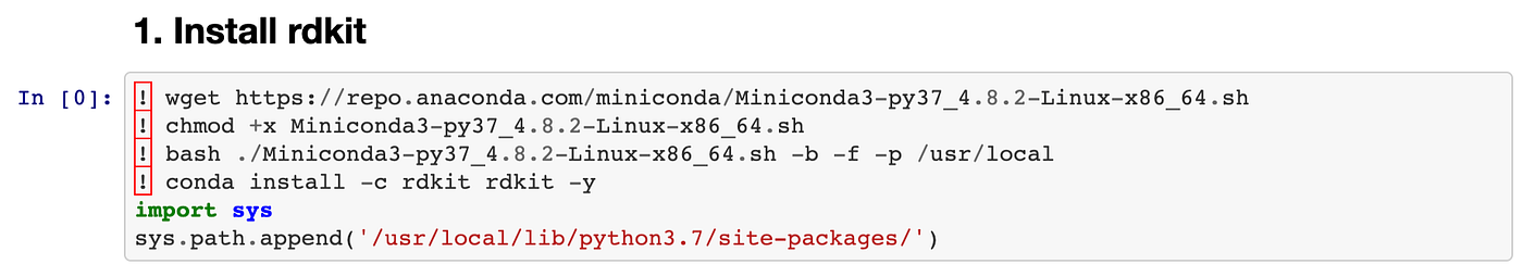
Rendering of the above 2 cells (text and code cell).
2.3. Data set
We will now download the Delaney solubility dataset that is available as a Supplementary file of the paper ESOL: Estimating Aqueous Solubility Directly from Molecular Structure.
Download data set
Download this into the Jupyter notebook as follows:
! wget https://raw.githubusercontent.com/dataprofessor/data/master/delaney.csv3. Methods
3.1. Dataset
3.1.1. Read in the dataset
Read in the CSV data that we had downloaded from the above cell. Assign the data into the sol dataframe.
import pandas as pd
sol = pd.read_csv('delaney.csv')
Displaying the sol dataframe gives us the following:
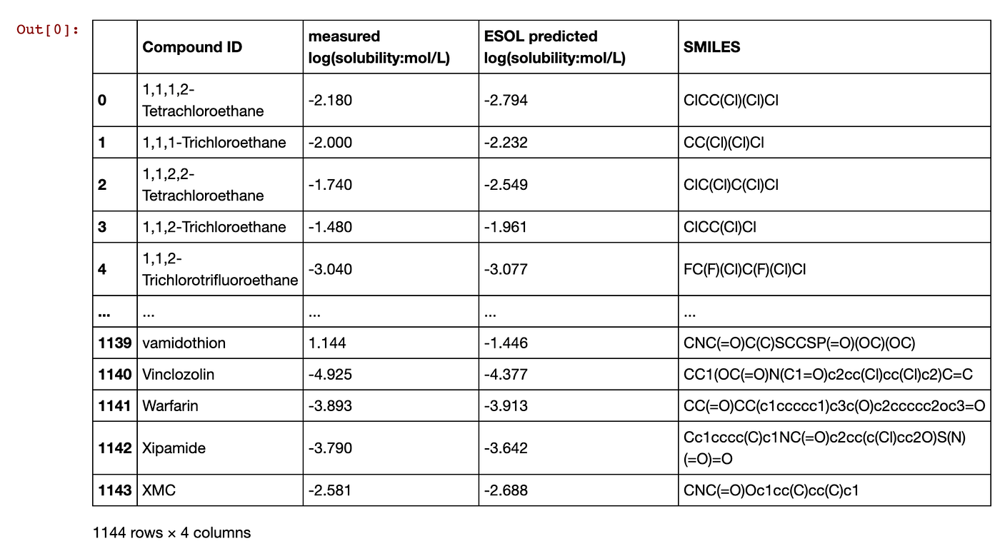
Contents of the sol dataframe.
3.1.2. Examining the SMILES data
Chemical structures are encoded by a string of text known as the SMILES notation which is an acronym for Simplified Molecular-Input Line-Entry System. Let’s have a look at the contents of the SMILES column from the sol dataframe.
sol.SMILESRunning the above cell will give us:
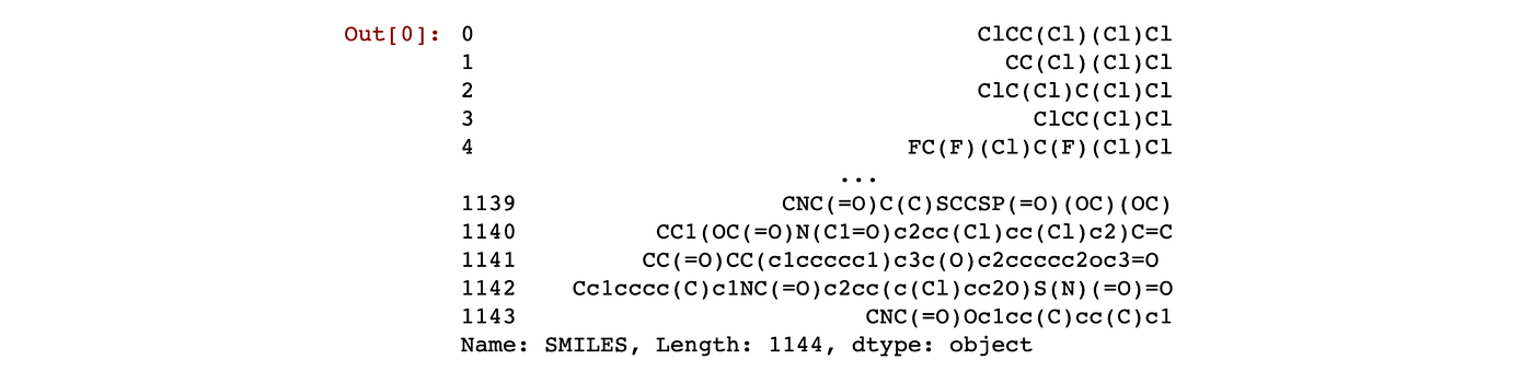
Contents of sol.SMILES (the SMILES column in the sol dataframe).
Each line represents a unique molecule. To select the first molecule (the first row), type sol.SMILES[0] and the output that we will see is ClCC(Cl)(Cl)Cl.
3.2. Working with SMILES string
3.2.1. Convert a molecule from the SMILES string to an rdkit object
Let’s start by importing the necessary library function:
from rdkit import Chem Now, apply the MolFromSmiles() function to convert the SMILES string to an rdkit molecule object:
Chem.MolFromSmiles(sol.SMILES[0])This will yield the output:
<rdkit.Chem.rdchem.Mol at 0x7f66f2e3e800>3.2.2. Working with the rdkit object
Let’s perform a simple count of the number of atoms on the query SMILES string, which we first convert to an rdkit object followed by applying the GetNumAtoms() function.
m = Chem.MolFromSmiles('ClCC(Cl)(Cl)Cl')
m.GetNumAtoms()
This produces an output of:
63.2.3. Convert list of molecules to rdkit object
But before we can do any descriptor calculation, we will first have to convert the SMILES string to rdkit object as mentioned above in section 3.2. Here we will do the same thing as described above but we will be making use of the for loop to iterate through the list of SMILES strings.
from rdkit import Chemmol_list= []
for element in sol.SMILES:
  mol = Chem.MolFromSmiles(element)
  mol_list.append(mol)
Next, we will check that the newly rdkit objects are populating the mol_list variable or not.
len(mol_list)The above line returns:
1144And this corresponds to 1,144 molecules. Now, we will have a look inside at the variable’s contents.
mol_list[:5]This yields the following output:
[<rdkit.Chem.rdchem.Mol at 0x7f66edb6d670>,
 <rdkit.Chem.rdchem.Mol at 0x7f66edb6d620>,
 <rdkit.Chem.rdchem.Mol at 0x7f66edb6d530>,
 <rdkit.Chem.rdchem.Mol at 0x7f66edb6d6c0>,
 <rdkit.Chem.rdchem.Mol at 0x7f66edb6d710>]
3.3. Calculate molecular descriptors
We will now represent each of the molecules in the dataset by a set of molecular descriptors that will be used for model building.
To predict LogS (log of the aqueous solubility), the study by Delaney makes use of 4 molecular descriptors:
cLogP (Octanol-water partition coefficient)
MW (Molecular weight)
RB (Number of rotatable bonds)
AP (Aromatic proportion = number of aromatic atoms / number of heavy atoms)
Unfortunately, rdkit readily computes the first 3. As for the AP descriptor, we will calculate this by manually computing the ratio of the number of aromatic atoms to the total number of heavy atoms which rdkit can compute.
3.3.1. Calculating LogP, MW and RB descriptors
We will now create a custom function called generate() for computing the 3 descriptors LogP, MW and RB.
import numpy as np
from rdkit.Chem import Descriptors# Inspired by: https://codeocean.com/explore/capsules?query=tag:data-curation

def generate(smiles, verbose=False):

    moldata= []
    for elem in smiles:
        mol=Chem.MolFromSmiles(elem)
        moldata.append(mol)

    baseData= np.arange(1,1)
    i=0
    for mol in moldata:

        desc_MolLogP = Descriptors.MolLogP(mol)
        desc_MolWt = Descriptors.MolWt(mol)
        desc_NumRotatableBonds = Descriptors.NumRotatableBonds(mol)

        row = np.array([desc_MolLogP,
                        desc_MolWt,
                        desc_NumRotatableBonds])

        if(i==0):
            baseData=row
        else:
            baseData=np.vstack([baseData, row])
        i=i+1

    columnNames=["MolLogP","MolWt","NumRotatableBonds"]
    descriptors = pd.DataFrame(data=baseData,columns=columnNames)

    return descriptors
Let’s apply the generate() function perform the actual descriptor calculation on sol.SMILES (the SMILES column from the df dataframe) and assign the descriptor output to the df variable.
df = generate(sol.SMILES)
df
The output of the df dataframe is shown below.
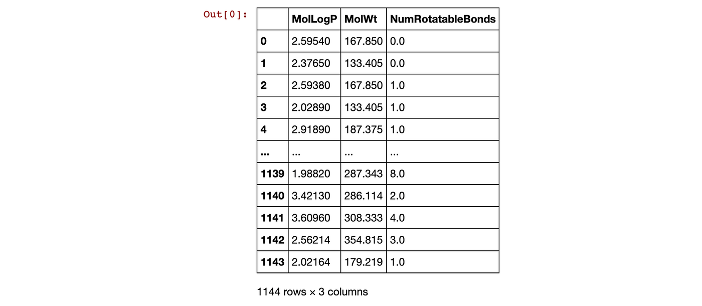
Contents of the df dataframe.
3.3.2. Calculating the aromatic proportion
As mentioned above, the equation for calculating the aromatic proportion is obtained by dividing the number of aromatic atoms by the number of heavy atoms.
3.3.2.1. Number of aromatic atoms
Here, we will create a custom function to calculate the Number of aromatic atoms. With this descriptor we can use it to subsequently calculate the AP descriptor.
Example for computing the number of aromatic atoms for a single molecule.
SMILES = 'COc1cccc2cc(C(=O)NCCCCN3CCN(c4cccc5nccnc54)CC3)oc21'm = Chem.MolFromSmiles(SMILES)aromatic_atoms = [m.GetAtomWithIdx(i).GetIsAromatic() for i in range(m.GetNumAtoms())]aromatic_atomsThis give the following output.
[False, False, True, True, True, True, True, True, True, False, False, False, False, False, False, False, False, False, False, False, True, True, True, True, True, True, True, True, True, True, False, False, True, True] Let’s now create a custom function called AromaticAtoms().
def AromaticAtoms(m):
  aromatic_atoms = [m.GetAtomWithIdx(i).GetIsAromatic() for i in range(m.GetNumAtoms())]
  aa_count = []
  for i in aromatic_atoms:
    if i==True:
      aa_count.append(1)
  sum_aa_count = sum(aa_count)
  return sum_aa_count
Now, apply the AromaticAtoms() function to compute the number of aromatic atoms for a query SMILES string.
AromaticAtoms(m)The output is:
19This means that there are 19 aromatic atoms (that is there are 19 atoms that are a part of aromatic rings).
Let’s now scale up and apply this to the entire SMILES list.
desc_AromaticAtoms = [AromaticAtoms(element) for element in mol_list]desc_AromaticAtomsNow, print out the results.
[0, 0, 0, 0, 0, 0, 0, 0, 6, 6, 6, 6, 6, 6, 6, 6, 6, 6, 6, 6, 6, 0, 6, 0, 0, 0, 0, 6, 6, 0, 6, 6, 6, 6, 6, 0, 6, 6, 0, 0, 6, 10, 6, 6, 0, 6, 6, 6, 6, 10, 6, 0, 10, 0, 14, 0, 0, 14, 0, 0, 0, 0, 10, 0, 0, 0, 0, 0, 0, 0, 0, 0, 0, 0, 10, 0, 0, 0, 0, 0, 10, 0, 0, 0, 0, ...]Congratulations! We now have computed the number of aromatic atoms for the entire dataset.
3.3.2.2. Number of heavy atoms
Here, we will use an existing function from the rdkit library for calculating the number of heavy atoms.
Example for computing the number of heavy atoms for a single molecule.
SMILES = 'COc1cccc2cc(C(=O)NCCCCN3CCN(c4cccc5nccnc54)CC3)oc21'
m = Chem.MolFromSmiles(SMILES)
Descriptors.HeavyAtomCount(m)
This yields the follow output.
34Let’s scale up to the entire SMILES list.
desc_HeavyAtomCount = [Descriptors.HeavyAtomCount(element) for element in mol_list]
desc_HeavyAtomCount
Now, print out the results.
[6, 5, 6, 5, 8, 4, 4, 8, 10, 10, 10, 9, 9, 10, 10, 10, 9, 9, 9, 8, 8, 4, 8, 4, 5, 8, 8, 10, 12, 4, 9, 9, 9, 15, 8, 4, 8, 8, 5, 8, 8, 12, 12, 8, 6, 8, 8, 10, 8, 12, 12, 5, 12, 6, 14, 11, 22, 15, 5, ...]3.3.2.3. Computing the aromatic proportion (AP) descriptor
Let’s now combine the number of aromatic atoms and the number of heavy atoms together.
Example of computing for a single molecule.
SMILES = 'COc1cccc2cc(C(=O)NCCCCN3CCN(c4cccc5nccnc54)CC3)oc21'
m = Chem.MolFromSmiles(SMILES)
AromaticAtoms(m)/Descriptors.HeavyAtomCount(m)
The output is:
0.5588235294117647Let’s scale up and compute for the entire SMILES list.
desc_AromaticProportion = [AromaticAtoms(element)/Descriptors.HeavyAtomCount(element) for element in mol_list]
desc_AromaticProportion
This gives the output:
[0.0, 0.0, 0.0, 0.0, 0.0, 0.0, 0.0, 0.0, 0.6, 0.6, 0.6, 0.6666666666666666, 0.6666666666666666, 0.6, 0.6, 0.6, 0.6666666666666666, 0.6666666666666666, 0.6666666666666666, 0.75, 0.75, 0.0, 0.75, 0.0, 0.0, 0.0, 0.0, 0.6, 0.5, 0.0, 0.6666666666666666, 0.6666666666666666, 0.6666666666666666, 0.4, 0.75, 0.0, 0.75, 0.75, 0.0, 0.0, 0.75, 0.8333333333333334, 0.5, 0.75, 0.0, 0.75, 0.75, 0.6, 0.75, 0.8333333333333334, 0.5, ...]Let’s now put this newly computed Aromatic Proportion descriptor into a dataframe.
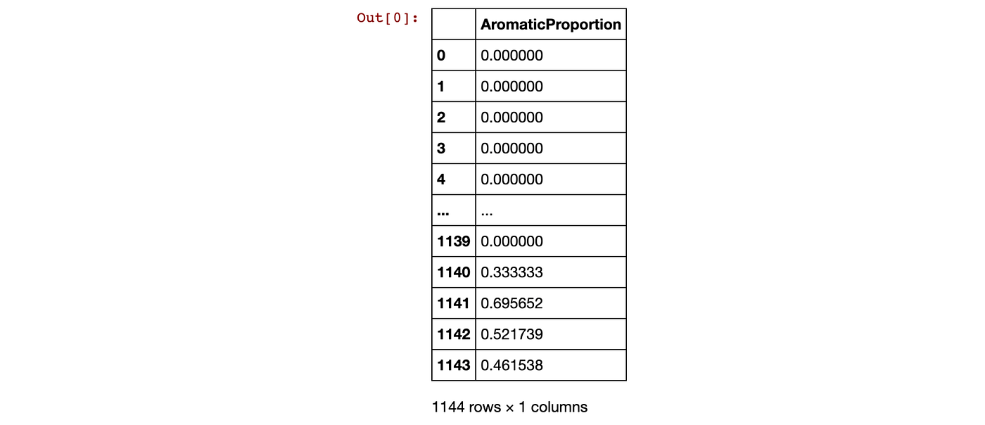
Contents of the Aromatic Proportion descriptor dataframe.
3.4. Dataset preparation
3.4.1. Creating the X matrix
Let’s combine all computed descriptors from 2 dataframe into 1 dataframe. Before doing that, let’s take a look at the 2 dataframes (df and df_desc_AromaticProportion) that we will be combining and how the combined dataframe will look like as illustrated below.
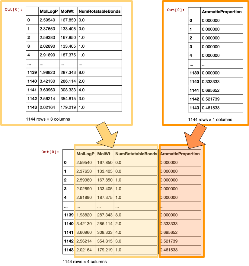
Illustration of combining the 2 descriptor-containing dataframes to form the X matrix.
Let’s actually combine the 2 dataframes to produce the X matrix.
X = pd.concat([df,df_desc_AromaticProportion], axis=1)
X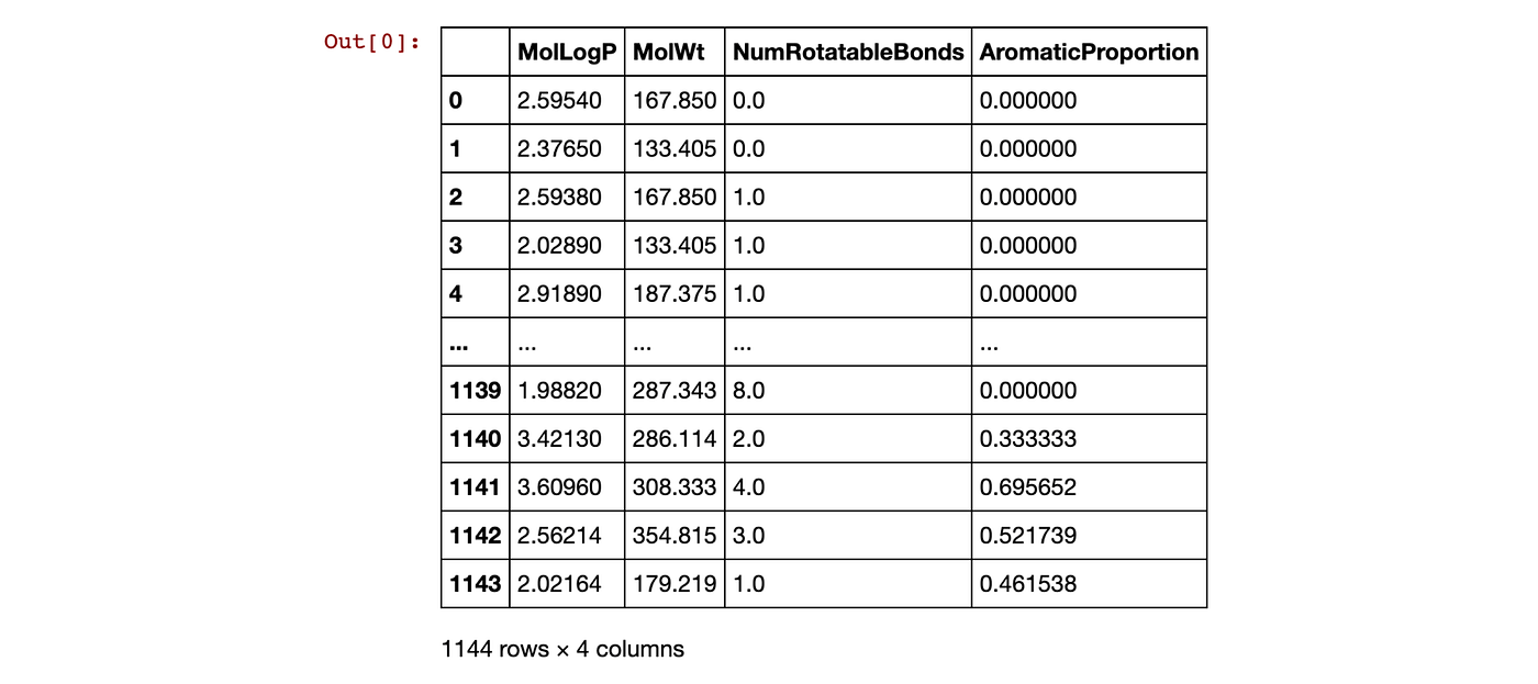
Contents of the X matrix dataframe created by combining 2 dataframes.
3.4.2. Creating the Y matrix
The Y matrix will be created from 1 column that we are going to predict in this tutorial and this is the LogS value. In the sol dataframe, the LogS values are contained within the measured log(solubility:mol/L) column.
Let’s have a look at the sol dataframe again.
sol.head()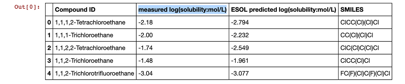
Contents of the sol dataframe with the LogS column highlighted.
The second column (index number of 1) corresponding to the measured solubility value (LogS) will be used as the Y matrix. Thus, we will select the second column (indicated in the above image by the blue highlight).
Y = sol.iloc[:,1]
Y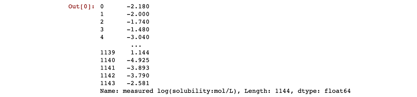
Contents of the Y matrix (LogS column).
3.5. Data split
We will now proceed to performing data splitting using a split ratio of 80/20 (i.e. we do this by assigning the test_size parameter to 0.2) whereby 80% of the initial dataset will be used as the training set and the remaining 20% of the dataset will be used as the testing set.
from sklearn.model_selection import train_test_splitX_train, X_test, Y_train, Y_test = train_test_split(X, Y,
                                                    test_size=0.2)
3.6. Linear regression model
As the original study by Delaney and the investigation by Walters used linear regression for model building, therefore for comparability we will also be using linear regression as well.
from sklearn import linear_model
from sklearn.metrics import mean_squared_error, r2_scoremodel = linear_model.LinearRegression()
model.fit(X_train, Y_train)
Upon running the above code block we will see the following output that essentially prints out the parameters used for model building.
LinearRegression(copy_X=True, fit_intercept=True, n_jobs=None, normalize=False)4. Results
4.1. Linear Regression Model
4.1.1. Predict the LogS value of X_train data
The trained model from section 3.6 will be applied here to predict the LogS values of all samples (the molecules) in the training set (X_train).
Y_pred_train = model.predict(X_train)print('Coefficients:', model.coef_)
print('Intercept:', model.intercept_)
print('Mean squared error (MSE): %.2f'
      % mean_squared_error(Y_train, Y_pred_train))
print('Coefficient of determination (R^2): %.2f'
      % r2_score(Y_train, Y_pred_train))
This generates the following prediction results.
Coefficients: [-0.7282008  -0.00691046  0.01625003 -0.35627645]
Intercept: 0.26284383753800666
Mean squared error (MSE): 0.99
Coefficient of determination (R^2): 0.77
Let’s analyse the above output line by line:
In the first line,
Coefficientslists the regression coefficient values of each independent variables (i.e. the 4 molecular descriptors consisting of LogP, MW, RB and AP)In the second line,
Interceptis essentially the y-intercept value where the regression line passes when X = 0.In the third line,
Mean squared error (MSE)is used as an error measure (i.e. the lower the better).In the fourth line,
Coefficient of determination (R²)is the squared value of Pearson’s correlation coefficient value and is used as a measure of goodness of fit for linear regression models (i.e. the higher the better)
4.1.2. Predict the LogS value of X_test data
Next, the trained model from section 3.6 will also be applied here to predict the LogS values of all samples (the molecules) in the training set (X_train).
We will print out the prediction performance as follows:
Y_pred_test = model.predict(X_test)print('Coefficients:', model.coef_)
print('Intercept:', model.intercept_)
print('Mean squared error (MSE): %.2f'
      % mean_squared_error(Y_test, Y_pred_test))
print('Coefficient of determination (R^2): %.2f'
      % r2_score(Y_test, Y_pred_test))
The above code block produces the following prediction results.
Coefficients: [-0.7282008  -0.00691046  0.01625003 -0.35627645]
Intercept: 0.26284383753800666
Mean squared error (MSE): 1.11
Coefficient of determination (R^2): 0.75
4.2. Comparing the Linear Regression Equation
The work of Delaney provided the following linear regression equation:
LogS = 0.16 - 0.63 cLogP - 0.0062 MW + 0.066 RB - 0.74 APThe reproduction by Pat Walters provided the following:
LogS = 0.26 - 0.74 LogP - 0.0066 MW + 0.0034 RB - 0.42 APThis tutorial’s reproduction gave the following equation:
Based on the Train set (shown below in section 4.3.1)
LogS = 0.26 - 0.73 LogP - 0.0069 MW 0.0163 RB - 0.36 APBased on the Full dataset (shown below in section 4.3.2)
LogS = 0.26 - 0.74 LogP - 0.0066 MW + 0.0032 RB - 0.42 AP4.3. Deriving the Linear Regression Equation
4.3.1. Based on the Train set
In the follow code block below we will be using the linear regression model constructed in section 3.6 whereby the Train set was used for model building. For your reference, I will put the code here:
from sklearn import linear_model
from sklearn.metrics import mean_squared_error, r2_scoremodel = linear_model.LinearRegression()
model.fit(X_train, Y_train)
Thus, we simply print out the equation directly from the previously built model contained within the model variable (i.e. by calling various columns of the model variable).
yintercept = '%.2f' % model.intercept_
LogP = '%.2f LogP' % model.coef_[0]
MW = '%.4f MW' % model.coef_[1]
RB = '%.4f RB' % model.coef_[2]
AP = '%.2f AP' % model.coef_[3]print('LogS = ' +
      ' ' +
      yintercept +
      ' ' +
      LogP +
      ' ' +
      MW +
      ' ' +
      RB +
      ' ' +
      AP)
Running the above code block gives the following equation output:
LogS = 0.26 -0.73 LogP -0.0069 MW 0.0163 RB -0.36 AP4.3.2. Based on the Full dataset (for comparison)
Here we will be using the entire dataset to train a linear regression model. The fit() function allows the defined model in full (i.e. the linear regression model) to be trained by using X and Y data matrices as the input argument.
full = linear_model.LinearRegression()
full.fit(X, Y)
This produces the following output:
LinearRegression(copy_X=True, fit_intercept=True, n_jobs=None, normalize=False)We will now print out the prediction performance.
full_pred = model.predict(X)print('Coefficients:', full.coef_)
print('Intercept:', full.intercept_)
print('Mean squared error (MSE): %.2f'
      % mean_squared_error(Y, full_pred))
print('Coefficient of determination (R^2): %.2f'
      % r2_score(Y, full_pred))
This generates the following output:
Coefficients: [-0.74173609 -0.00659927  0.00320051 -0.42316387]
Intercept: 0.2565006830997185
Mean squared error (MSE): 1.01
Coefficient of determination (R^2): 0.77
Finally, we will print out the linear regression equation.
full_yintercept = '%.2f' % full.intercept_
full_LogP = '%.2f LogP' % full.coef_[0]
full_MW = '%.4f MW' % full.coef_[1]
full_RB = '+ %.4f RB' % full.coef_[2]
full_AP = '%.2f AP' % full.coef_[3]print('LogS = ' +
      ' ' +
      full_yintercept +
      ' ' +
      full_LogP +
      ' ' +
      full_MW +
      ' ' +
      full_RB +
      ' ' +
      full_AP)
This yields the following output.
LogS = 0.26 -0.74 LogP -0.0066 MW + 0.0032 RB -0.42 AP4.4. Scatter plot of experimental vs. predicted LogS
Before beginning, let’s do a quick check of the variable dimensions of Train and Test sets.
Here we are checking the dimension of the Train set.
Y_train.shape, Y_pred_train.shapeThis produces the following dimension output:
((915,), (915,))Here we are checking the dimension of the Test set.
Y_test.shape, Y_pred_test.shapeThis produces the following dimension output:
((229,), (229,))4.4.1. Vertical Plot
Let’s now visualise the correlation of the Experimental LogS values with those of the Predicted LogS values by means of the scatter plot. We will be displaying the Experimental vs Predicted values of LogS separately in 2 scatter plots. In this first version, we will be stacking the 2 scatter plots vertically.
import matplotlib.pyplot as pltplt.figure(figsize=(5,11))

# 2 row, 1 column, plot 1
plt.subplot(2, 1, 1)
plt.scatter(x=Y_train, y=Y_pred_train, c="#7CAE00", alpha=0.3)

# Add trendline
# https://stackoverflow.com/questions/26447191/how-to-add-trendline-in-python-matplotlib-dot-scatter-graphs
z = np.polyfit(Y_train, Y_pred_train, 1)
p = np.poly1d(z)
plt.plot(Y_test,p(Y_test),"#F8766D")

plt.ylabel('Predicted LogS')


# 2 row, 1 column, plot 2
plt.subplot(2, 1, 2)
plt.scatter(x=Y_test, y=Y_pred_test, c="#619CFF", alpha=0.3)

z = np.polyfit(Y_test, Y_pred_test, 1)
p = np.poly1d(z)
plt.plot(Y_test,p(Y_test),"#F8766D")

plt.ylabel('Predicted LogS')
plt.xlabel('Experimental LogS')

plt.savefig('plot_vertical_logS.png')
plt.savefig('plot_vertical_logS.pdf')
plt.show()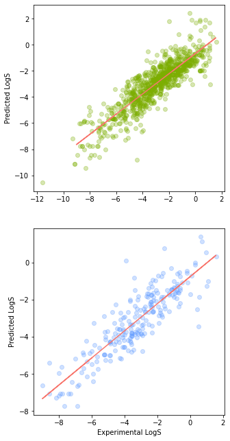
Scatter Plot of the Predicted vs Experimental LogS values (shown as a Vertical Plot).
4.4.2. Horizontal Plot
In this second version, we will be laying the 2 scatter plots horizontally as shown in the following code block.
import matplotlib.pyplot as pltplt.figure(figsize=(11,5))
vf
# 1 row, 2 column, plot 1
plt.subplot(1, 2, 1)
plt.scatter(x=Y_train, y=Y_pred_train, c="#7CAE00", alpha=0.3)

z = np.polyfit(Y_train, Y_pred_train, 1)
p = np.poly1d(z)
plt.plot(Y_test,p(Y_test),"#F8766D")

plt.ylabel('Predicted LogS')
plt.xlabel('Experimental LogS')

# 1 row, 2 column, plot 2
plt.subplot(1, 2, 2)
plt.scatter(x=Y_test, y=Y_pred_test, c="#619CFF", alpha=0.3)

z = np.polyfit(Y_test, Y_pred_test, 1)
p = np.poly1d(z)
plt.plot(Y_test,p(Y_test),"#F8766D")

plt.xlabel('Experimental LogS')

plt.savefig('plot_horizontal_logS.png')
plt.savefig('plot_horizontal_logS.pdf')
plt.show()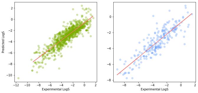
Scatter Plot of the Predicted vs Experimental LogS values (shown as a Horizontal Plot).
Cover image customised a Graphics (with license) by wowomnom on Envato Elements